Day 10: Data Augmentation With Fashion MNIST

Day 10 is all about data augmentation, a great way to improve the performance and generalizability of your model. Let’s dive into the Fashion MNIST dataset and apply data augmentation using Keras.

Overview of Data Augmentation

• Data Augmentation is a technique used to artificially expand the size of a training dataset by applying random transformations like rotation, shifting, flipping, and zooming to the existing images.
• This helps improve the robustness of your model by exposing it to more variations, thereby reducing overfitting.
• Fashion MNIST: This dataset contains grayscale images of clothing items, with 10 classes like shirts, trousers, bags, etc.

Goal of Today’s Task

1. Load the Fashion MNIST dataset.
2. Build a CNN model.
3. Use Keras’s pre-built data augmentation methods to generate more diverse training images.
4. Train the model with augmented data to see the difference in performance.

Step-by-Step Implementation

Step 1: Import Libraries and Load Dataset

We start by importing the necessary libraries and loading the Fashion MNIST dataset.

import tensorflow as tf
from tensorflow.keras.models import Sequential
from tensorflow.keras.layers import Conv2D, MaxPooling2D, Flatten, Dense
from tensorflow.keras.layers import Dropout
from tensorflow.keras.datasets import fashion_mnist
from tensorflow.keras.preprocessing.image import ImageDataGenerator
import matplotlib.pyplot as plt

# Load the Fashion MNIST dataset
(X_train, y_train), (X_test, y_test) = fashion_mnist.load_data()

# Display the shape of the data
print('Training data shape:', X_train.shape)
print('Test data shape:', X_test.shape)

Explanation:

• Fashion MNIST Dataset: Contains grayscale images of various clothing items, each with a shape of 28x28 pixels.
• Train and Test Split: The dataset is pre-split into training and test sets, making it easy to use.

Step 2: Preprocess the Data

We need to normalize the images and reshape them for the model.

Explanation:

• Reshape: Adds an extra dimension for channels. Since the images are grayscale, there’s only 1 channel.
• Normalization: Scales pixel values between 0 and 1, which speeds up training and enhances model effectiveness.

# Reshape the data to add the channel dimension (grayscale has 1 channel)
X_train = X_train.reshape(X_train.shape[0], 28, 28, 1)
X_test = X_test.reshape(X_test.shape[0], 28, 28, 1)

# Normalize pixel values to be between 0 and 1
X_train = X_train.astype('float32') / 255.0
X_test = X_test.astype('float32') / 255.0

Step 3: Apply Data Augmentation Using ImageDataGenerator

We will use Keras’s ImageDataGenerator class to apply data augmentation.

# Create an ImageDataGenerator with data augmentation settings
datagen = ImageDataGenerator(
    rotation_range=15,          # Rotate the image by up to 15 degrees
    width_shift_range=0.1,      # Shift the width by up to 10% of the image width
    height_shift_range=0.1,     # Shift the height by up to 10% of the image height
    zoom_range=0.1,             # Zoom in by up to 10%
    horizontal_flip=True        # Randomly flip images horizontally
)

# Fit the ImageDataGenerator to the training data
datagen.fit(X_train)

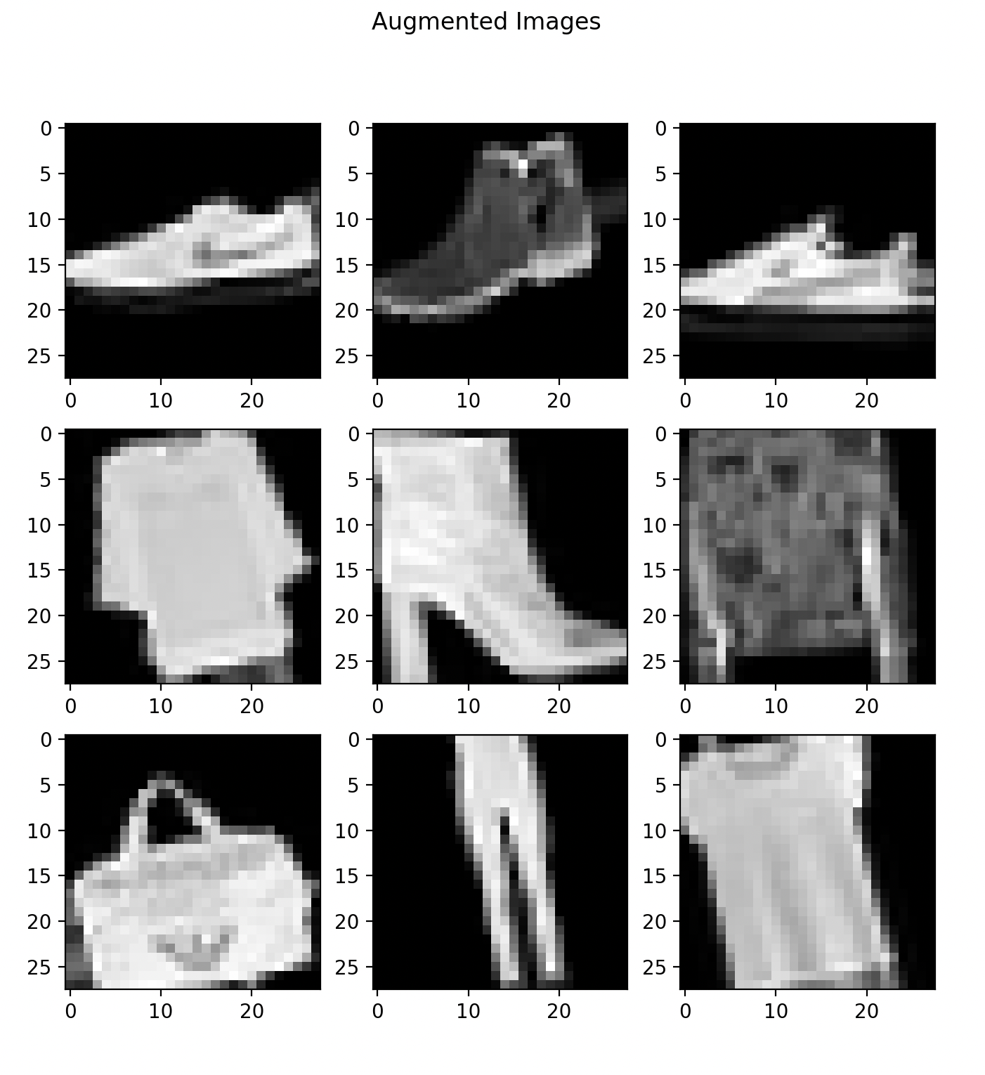
# Let's visualize some augmented images
for X_batch, y_batch in datagen.flow(X_train, y_train, batch_size=9):
    # Create a grid of 3x3 images
    fig, ax = plt.subplots(3, 3, figsize=(8, 8))
    for i in range(9):
        ax[i//3, i%3].imshow(X_batch[i].reshape(28, 28), cmap='gray')
        ax[i//3, i%3].axis('off')
    plt.suptitle('Augmented Images')
    plt.show()
    break  # Only show one batch

Explanation:

• ImageDataGenerator:
  • rotation_range=15: Rotates images randomly by up to 15 degrees.
  • width_shift_range=0.1 and height_shift_range=0.1: Shifts images horizontally or vertically by 10% of the image dimensions.
  • zoom_range=0.1: Randomly zooms in by up to 10%.
  • horizontal_flip=True: Randomly flips images horizontally.
• datagen.flow(): Generates batches of augmented images. We visualize a 3x3 grid of augmented images for a better understanding of how augmentation works.

Step 4: Define the CNN Model

We’ll create a CNN model to classify images in the Fashion MNIST dataset.

# Define the CNN model
model = Sequential()

# Convolutional Layer 1
model.add(Conv2D(32, (3, 3), activation='relu', input_shape=(28, 28, 1)))
model.add(MaxPooling2D((2, 2)))

# Convolutional Layer 2
model.add(Conv2D(64, (3, 3), activation='relu'))
model.add(MaxPooling2D((2, 2)))

# Flatten the output to feed into fully connected layers
model.add(Flatten())

# Fully Connected Layer
model.add(Dense(128, activation='relu'))
model.add(Dropout(0.5))

# Output Layer
model.add(Dense(10, activation='softmax'))

# Compile the model
model.compile(optimizer='adam', loss='categorical_crossentropy', metrics=['accuracy'])

# Summary of the model
model.summary()

Explanation:

• Convolutional Layers: The first layer has 32 filters, and the second layer has 64 filters, enabling the model to learn different features.
• MaxPooling2D: Reduces the size of feature maps, allowing the model to focus on prominent features.
• Fully Connected Layer: A layer with 128 neurons, followed by a Dropout layer with a 50% dropout rate to prevent overfitting.
• Output Layer: Has 10 neurons (for the 10 classes in Fashion MNIST) with softmax activation to produce class probabilities.

Step 5: Train the Model with Augmented Data

Now, we’ll train the model using the augmented images generated by ImageDataGenerator.

# Train the model using the augmented data
history = model.fit(datagen.flow(X_train, y_train, batch_size=64),
                    validation_data=(X_test, y_test),
                    epochs=15, verbose=1)

Explanation:

• datagen.flow(X_train, y_train, batch_size=64): Generates batches of augmented data on-the-fly during training.
• Validation Data: The test set is used for evaluation after each epoch.
• Epochs: The model is trained for 15 epochs, giving it enough time to learn from the augmented data.

Step 6: Visualize Training Performance

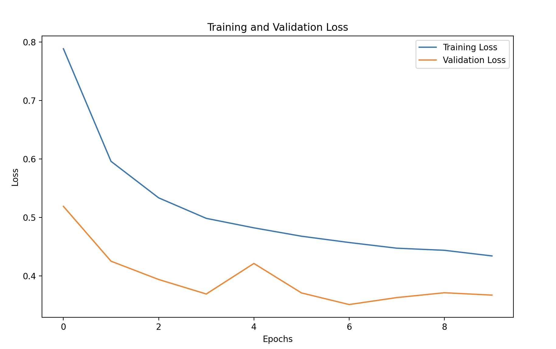
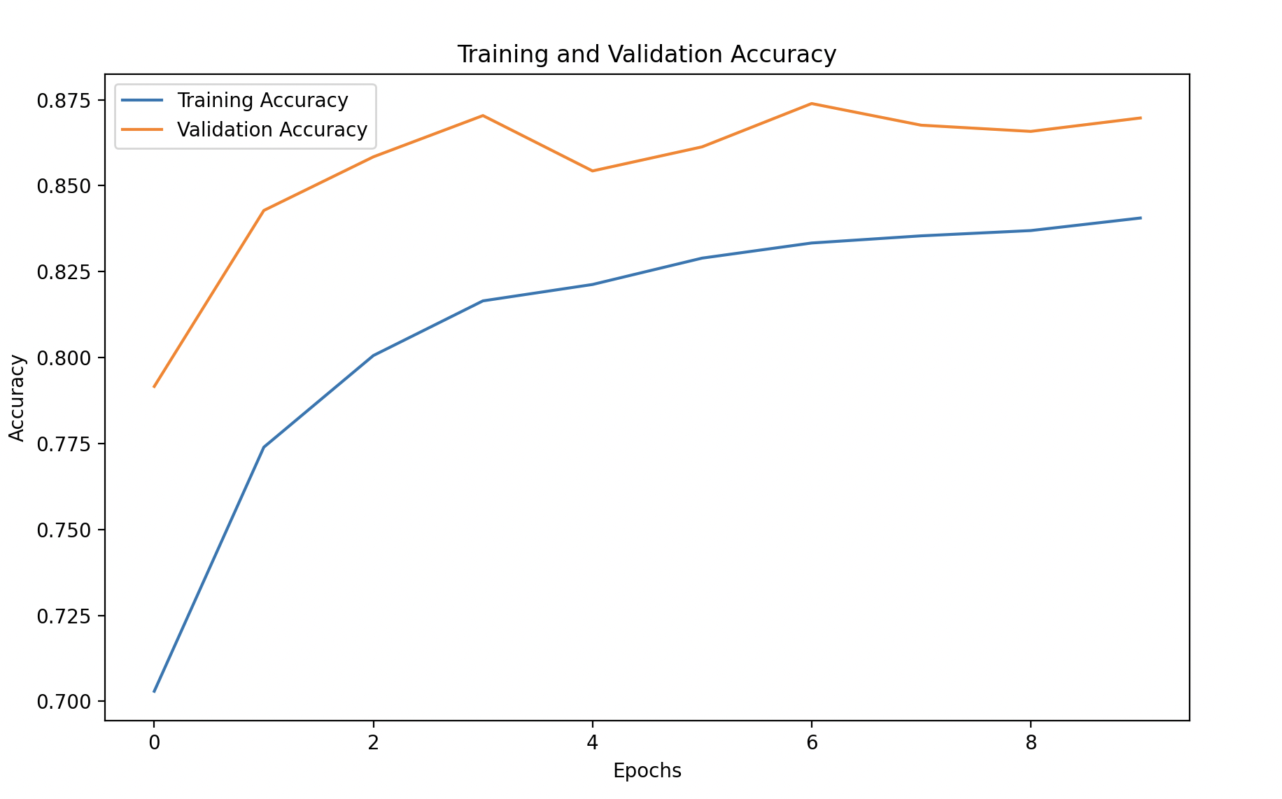
We’ll plot the training and validation accuracy and loss to monitor the model’s performance over time.

import pandas as pd

# Convert the history to a DataFrame for easy visualization
history_df = pd.DataFrame(history.history)

# Plot training and validation accuracy
plt.figure(figsize=(10, 6))
plt.plot(history_df['accuracy'], label='Training Accuracy')
plt.plot(history_df['val_accuracy'], linestyle='--', label='Validation Accuracy')
plt.xlabel('Epochs')
plt.ylabel('Accuracy')
plt.title('Training and Validation Accuracy')
plt.legend()
plt.show()

# Plot training and validation loss
plt.figure(figsize=(10, 6))
plt.plot(history_df['loss'], label='Training Loss')
plt.plot(history_df['val_loss'], linestyle='--', label='Validation Loss')
plt.xlabel('Epochs')
plt.ylabel('Loss')
plt.title('Training and Validation Loss')
plt.legend()
plt.show()

Explanation:

• Training vs. Validation Accuracy/Loss: This helps identify if the model is overfitting or generalizing well to unseen data. Ideally, both accuracy metrics should increase, and both loss metrics should decrease.

Key Points About Data Augmentation

More Data Without Collecting New Images

• Data augmentation helps generate more diverse data from the existing dataset.
• You don’t need to collect additional images; you simply create variations from the ones you have.

Improves Generalization

• The model learns to recognize features even when they are rotated, shifted, flipped, or zoomed.
• This enhances the model’s ability to generalize and perform better on unseen data.

Reduces Overfitting

• Augmentation prevents the model from simply memorizing the training data by introducing more variety.
• As a result, the model learns robust patterns rather than memorizing specific examples.

Video