Day 2: Classify Handwritten Digits Using a Simple NN on MNIST

The MNIST dataset is one of the most popular datasets for learning the basics of machine learning and neural networks. It contains handwritten digits (0-9), and our goal is to build a neural network that can classify these digits.

We’ll use a Simple Neural Network (i.e., a Feedforward Neural Network) for this task. Let’s break down the solution into easy-to-follow steps, and I’ll explain every part so you understand what’s happening. We will use Keras, a high-level API in TensorFlow, to make this as simple as possible.

Step-by-Step Solution Outline:

1. Load the MNIST Dataset.
2. Prepare and Preprocess the Data.
3. Build a Simple Feedforward Neural Network.
4. Compile and Train the Model.
5. Evaluate the Model Performance.
6. Make Predictions (optional step to visualize some predictions).

Here’s the full code along with detailed explanations:

Step-by-Step Implementation

Step 1: Import Libraries and Load Data

import numpy as np
import tensorflow as tf
from tensorflow.keras.datasets import mnist
from tensorflow.keras.models import Sequential
from tensorflow.keras.layers import Dense, Flatten
import matplotlib.pyplot as plt

• numpy: Used for numerical operations.
• tensorflow: We’ll use Keras, which is a part of TensorFlow, to create our neural network.
• mnist: The MNIST dataset is built into Keras, which makes it easy to load.
• Sequential and Dense: These help in building a neural network. Sequential is used for stacking layers.
• matplotlib: Used for visualizing the digits from the dataset.

Step 2: Load the MNIST Dataset

# Load the MNIST dataset
(X_train, y_train), (X_test, y_test) = mnist.load_data()

# Check the shape of the data
print(f"Training data shape: {X_train.shape}, Training labels shape: {y_train.shape}")
print(f"Testing data shape: {X_test.shape}, Testing labels shape: {y_test.shape}")

• mnist.load_data() loads the MNIST data and splits it into training and testing sets.
  • X_train: Images of handwritten digits used for training the model.
  • y_train: Corresponding labels for the training images (digits 0-9).
  • X_test and y_test are the images and labels used for testing.
• Shapes:
  • X_train.shape: The shape is (60000, 28, 28), which means we have 60,000 images, each with a size of 28x28 pixels.
  • y_train.shape: We have 60,000 labels corresponding to the training images.

Step 3: Preprocess the Data

# Normalize the data to range 0-1
X_train = X_train / 255.0
X_test = X_test / 255.0

# Flatten the images from 28x28 to 784 (since a dense layer expects a vector input)
X_train = X_train.reshape(-1, 28 * 28)
X_test = X_test.reshape(-1, 28 * 28)

• Normalize the Data:
  • X_train / 255.0: The original pixel values are between 0 and 255. Dividing by 255 scales these values to between 0 and 1, which helps the neural network learn faster.
• Flatten the Images:
  • The MNIST images are 28x28 pixels, which we need to flatten into a vector of 784 pixels (28 * 28). This is because a fully connected (Dense) layer expects 1D vectors rather than 2D images.

Step 4: Build the Neural Network

# Build a simple feedforward neural network model
model = Sequential()
model.add(Dense(128, activation='relu', input_shape=(784,)))  # First hidden layer with 128 neurons
model.add(Dense(64, activation='relu'))                       # Second hidden layer with 64 neurons
model.add(Dense(10, activation='softmax'))                    # Output layer with 10 neurons (for digits 0-9)

• Sequential(): We create a Sequential model to stack layers one after another.
• Dense(128, activation=‘relu’, input_shape=(784,)): 128 neurons in the first hidden layer with ReLU activation function.
  • input_shape=(784,) tells the model that the input will be a vector of length 784 (flattened image).
  • Dense(64, activation=‘relu’): Adds a second hidden layer with 64 neurons and ReLU activation.
• Dense(10, activation=‘softmax’): The output layer has 10 neurons, each representing one of the digits 0-9.
  • softmax activation is used to turn the output into probabilities, with the sum equal to 1.

Step 5: Compile the Model

model.compile(optimizer='adam', loss='sparse_categorical_crossentropy', metrics=['accuracy'])

• optimizer=‘adam’: The Adam optimizer is a popular choice for training deep learning models.
• loss=‘sparse_categorical_crossentropy’: We use categorical cross-entropy since we have multiple classes (0-9) to predict. Sparse is used since our labels are integers (0-9) rather than one-hot encoded vectors.
• metrics=[‘accuracy’]: We use accuracy to track the model’s performance during training and testing.

Step 6: Train the Model

history = model.fit(X_train, y_train, validation_data=(X_test, y_test), epochs=10, batch_size=32, verbose=1)

• model.fit(): Train the model using the training data.
  • validation_data=(X_test, y_test): Evaluate performance on the testing data during training.
  • epochs=10: Train for 10 complete passes through the training dataset.
  • batch_size=32: Update weights after every 32 samples.
  • verbose=1: Print detailed information during training.

Step 7: Evaluate the Model

test_loss, test_accuracy = model.evaluate(X_test, y_test)
print(f"Test Accuracy: {test_accuracy:.2f}")

• model.evaluate(X_test, y_test): Evaluates the model’s performance on the test data.
• test_accuracy: This gives us an idea of how well the model can classify unseen handwritten digits.

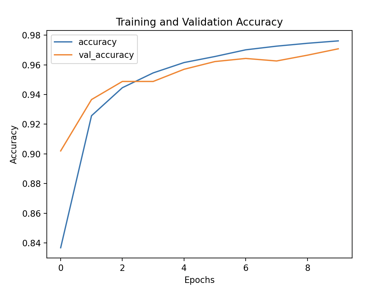
Step 8: Visualize Training and Validation Performance (Optional)

# Convert history to DataFrame and plot accuracy and loss
history_df = pd.DataFrame(history.history)
history_df[['accuracy', 'val_accuracy']].plot()
plt.xlabel('Epochs')
plt.ylabel('Accuracy')
plt.title('Training and Validation Accuracy')
plt.show()

• pd.DataFrame(history.history): Converts the training history to a DataFrame for easy visualization.
• Plotting:
  • Training and validation accuracy are plotted to see if the model’s performance improves over epochs and whether it overfits or underfits.

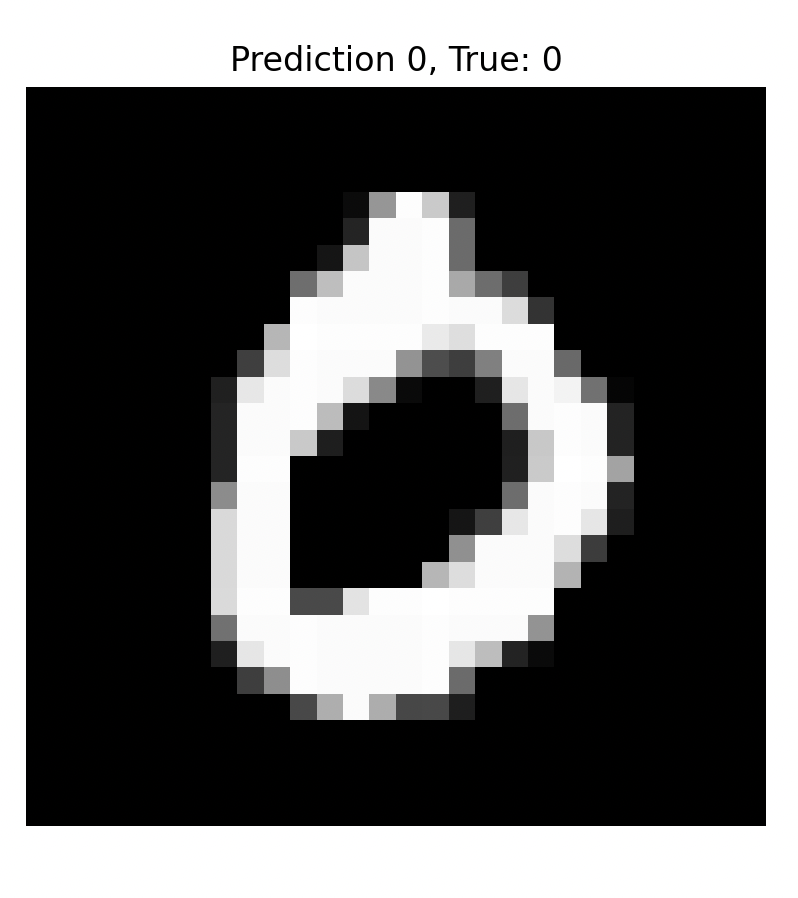
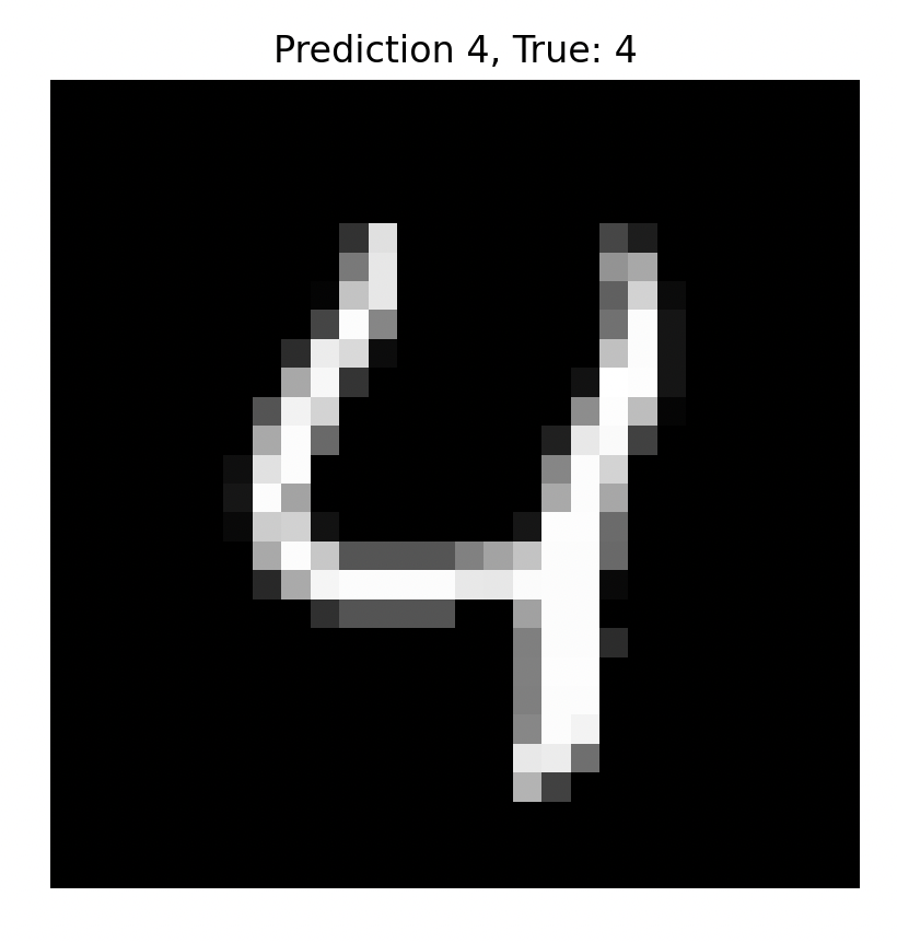
Step 9 (Optional): Make Some Predictions

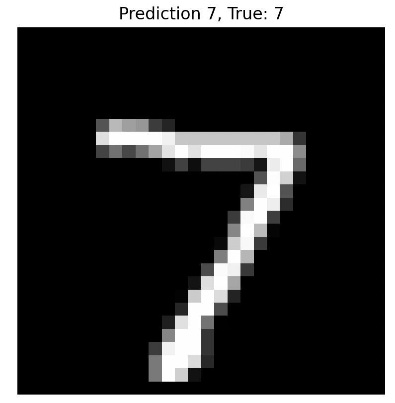
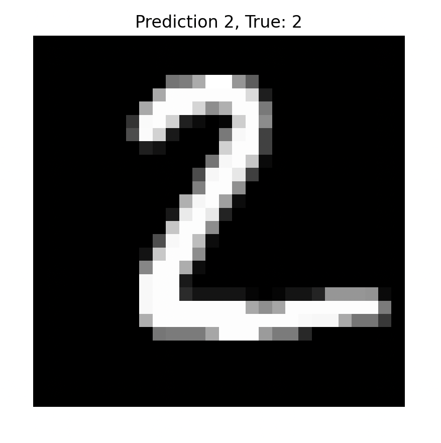
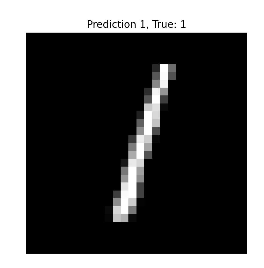
# Make predictions on the first 5 test images
predictions = model.predict(X_test[:5])

# Display the first 5 images with predicted and true labels
for i in range(5):
    plt.imshow(X_test[i].reshape(28, 28), cmap='gray')
    plt.title(f"Predicted: {np.argmax(predictions[i])}, True: {y_test.iloc[i]}")
    plt.axis('off')
    plt.show()

• model.predict(X_test[:5]): Predicts the labels for the first 5 test images.
• plt.imshow(): Displays each of the test images.
• np.argmax(predictions[i]): Retrieves the predicted label for each image.
• y_test.iloc[i]: Shows the true label.

Video

Coming Soon.