Day 3: Explore Backpropagation Theory and Tweak Learning Rates (MNIST)

What is Backpropagation?

Backpropagation is the algorithm that makes neural networks learn by adjusting their weights. Essentially, it’s the learning process.

It works by calculating the error in predictions (the difference between predicted and true values) and then propagating this error backward through the network to update the weights in each layer so that the model can make better predictions in the future.

How Backpropagation Works in Simple Terms:

• Forward Pass: The input data is passed through the network layer by layer to produce an output.
• Calculate Loss: The output is compared to the actual labels to calculate the loss (the error).
• Backward Pass (Gradient Calculation): The loss is used to compute the gradient of the error with respect to each weight.
• Weight Update: The weights are updated in the direction that minimizes the loss using the gradient and a learning rate.

Learning Rate: What Does It Do?

• The learning rate controls how big of a step we take in the direction of minimizing the error.
• High Learning Rate: Faster learning but might overshoot the minimum and miss convergence.
• Low Learning Rate: More stable, but can be slow and get stuck in local minima.

Today, we’ll experiment with different learning rates to see their effect on training.

Let’s Explore Practically with MNIST

We’ll modify our MNIST classifier and test different learning rates to observe the impact. Here’s how we’ll proceed:

1. Load the MNIST Dataset.
2. Build the neural network.
3. Compile the model with different learning rates.
4. Train the model and observe how changing learning rates impacts the training process.
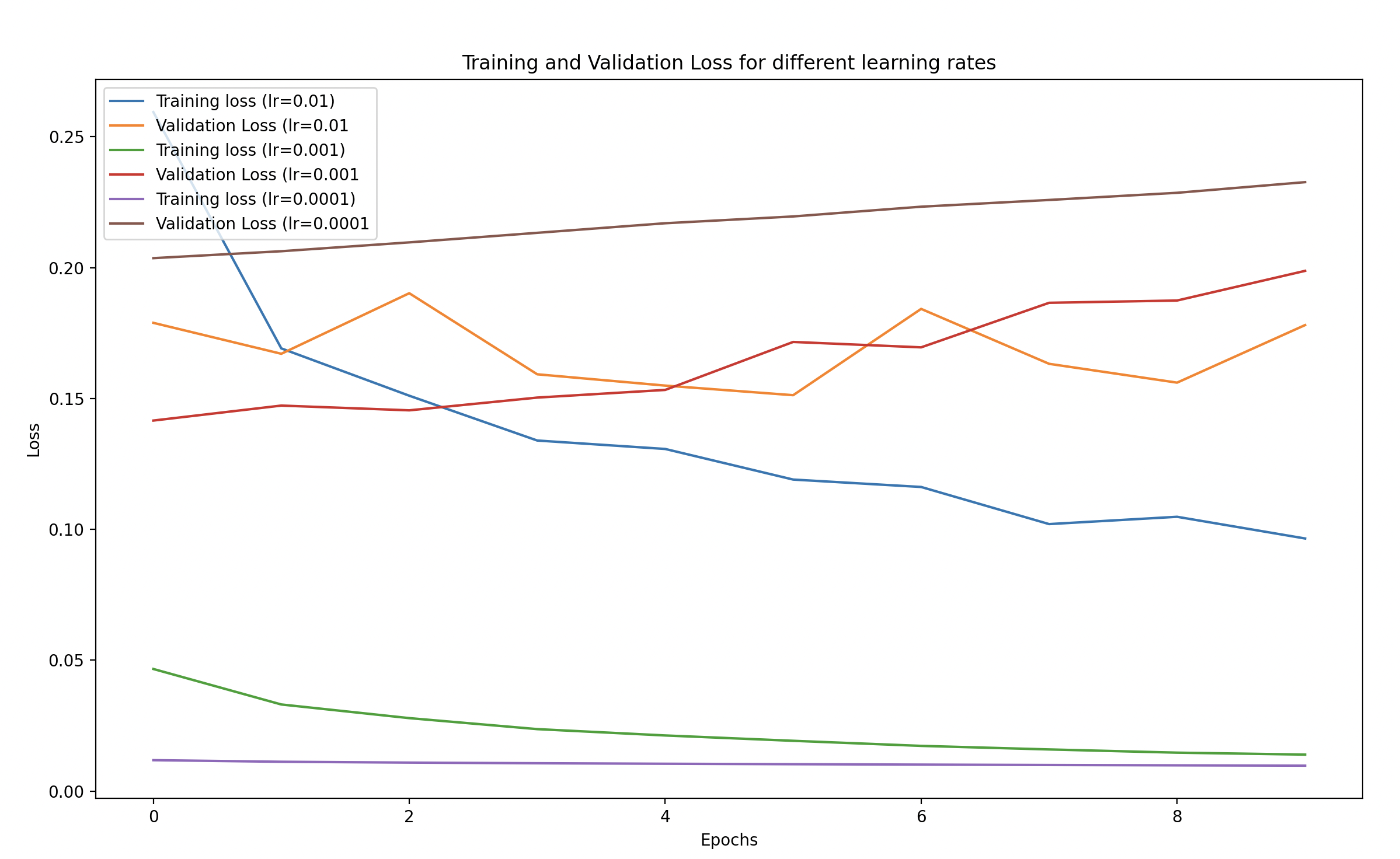
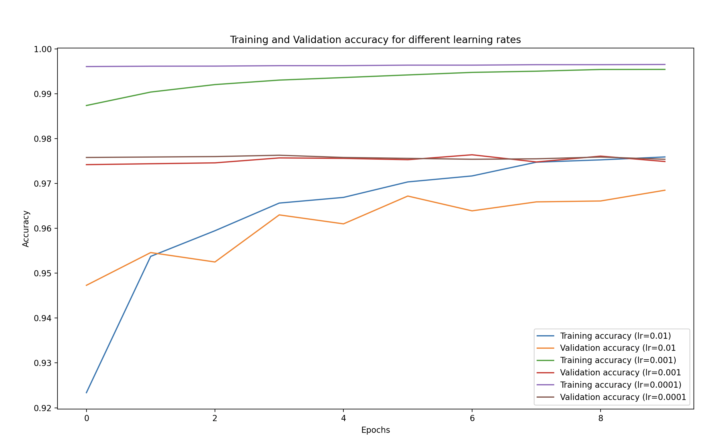
5. Plot the training and validation accuracy/loss to visualize the effect of different learning rates.

Here’s the full code along with detailed explanations:

Step-by-Step Implementation

Step 1: Load Libraries and the MNIST Dataset

import numpy as np
import pandas as pd
import tensorflow as tf
from tensorflow.keras.datasets import mnist
from tensorflow.keras.models import Sequential
from tensorflow.keras.layers import Dense, Flatten
import matplotlib.pyplot as plt

# Load the MNIST dataset
(X_train, y_train), (X_test, y_test) = mnist.load_data()

# Normalize the data to range 0-1
X_train = X_train / 255.0
X_test = X_test / 255.0

Libraries:

• numpy: Used for numerical operations.
• tensorflow: We’ll use Keras, which is a part of TensorFlow, to create our neural network.
• mnist: The MNIST dataset is built into Keras, which makes it easy to load.
• Sequential and Dense: These help in building a neural network. Sequential is used for stacking layers.
• matplotlib: Used for visualizing the digits from the dataset.

We load the data and then normalize the pixel values between 0 and 1 to improve the training process.

Step 2: Build the Neural Network Model

# Build a simple feedforward neural network model
model = Sequential()
model.add(Flatten(input_shape=(28, 28)))  # Flatten the 28x28 images to 784-length vectors
model.add(Dense(128, activation='relu'))  # First hidden layer with 128 neurons
model.add(Dense(64, activation='relu'))   # Second hidden layer with 64 neurons
model.add(Dense(10, activation='softmax'))  # Output layer with 10 neurons (for digits 0-9)

• We use a Flatten layer to convert the 28x28 image into a 1D vector.
• Then, we use Dense layers with ReLU activation for learning complex patterns.
• The output layer uses softmax to produce a probability distribution over 10 classes (digits 0-9).

Step 3: Experiment with Different Learning Rates

Now we’ll create multiple versions of the same model but with different learning rates:

# Different learning rates to experiment with
learning_rates = [0.01, 0.001, 0.0001]

# Store training history for each learning rate
history_dict = {}

for lr in learning_rates:
    # Compile the model with a specific learning rate
    model.compile(optimizer=tf.keras.optimizers.Adam(learning_rate=lr),
                  loss='sparse_categorical_crossentropy',
                  metrics=['accuracy'])

    # Train the model
    print(f"Training with learning rate: {lr}")
    history = model.fit(X_train, y_train, validation_data=(X_test, y_test),
                        epochs=10, batch_size=32, verbose=1)

    # Save the history for plotting
    history_dict[lr] = history.history

• Learning Rates: We’re testing with three different values:
  • 0.01: High learning rate.
  • 0.001: Standard default learning rate.
  • 0.0001: Low learning rate
• Loop through Learning Rates:
  • We compile and train the model for each learning rate.
  • optimizer=tf.keras.optimizers.Adam(learning_rate=lr) allows us to use the Adam optimizer with a specific learning rate.
  • history_dict[lr] saves the training history for later comparison.

Step 4: Visualize the Effect of Different Learning Rates

After training, we can visualize the training and validation accuracy and loss for different learning rates to see their impact:

# Plot training and validation loss for different learning rates
plt.figure(figsize=(14, 8))

for lr in learning_rates:
    plt.plot(history_dict[lr]['loss'], label=f'Training Loss (lr={lr})')
    plt.plot(history_dict[lr]['val_loss'], linestyle='--', label=f'Validation Loss (lr={lr})')

plt.xlabel('Epochs')
plt.ylabel('Loss')
plt.title('Training and Validation Loss for Different Learning Rates')
plt.legend()
plt.show()

# Plot training and validation accuracy for different learning rates
plt.figure(figsize=(14, 8))

for lr in learning_rates:
    plt.plot(history_dict[lr]['accuracy'], label=f'Training Accuracy (lr={lr})')
    plt.plot(history_dict[lr]['val_accuracy'], linestyle='--', label=f'Validation Accuracy (lr={lr})')

plt.xlabel('Epochs')
plt.ylabel('Accuracy')
plt.title('Training and Validation Accuracy for Different Learning Rates')
plt.legend()
plt.show()

• We plot the training and validation loss as well as accuracy for each learning rate.
• This will help us visually understand how different learning rates affect the training process.

Observations

Learning Rate Effects:

• High Learning Rate (0.01):
  • Likely unstable, as it makes large steps towards the minimum of the loss function, potentially overshooting.
  • You may notice fluctuating or diverging losses and unstable accuracy.
• Default Learning Rate (0.001):
  • Often results in a good balance between fast convergence and stability.
  • Training and validation loss will gradually decrease, and accuracy will steadily improve.
• Low Learning Rate (0.0001):
  • Training will be much slower, and the model might take a lot of time to converge.
  • Loss might decrease very gradually, and you might see the accuracy improving slowly, which could lead to longer training times.

Video

Coming Soon.