Day 4: Compare Activation Functions (ReLU, Sigmoid, Tanh) on Fashion MNIST
Comparing activation functions is key to understanding how they influence a neural network’s ability to learn and generalize. Today, we’ll explore the Fashion MNIST dataset and compare the effect of different activation functions: ReLU, Sigmoid, and Tanh on the model’s performance.
Problem Outline
- We’ll train multiple neural network models on the Fashion MNIST dataset.
- We will vary the activation functions used in the hidden layers: ReLU, Sigmoid, and Tanh.
- We will observe how each activation function affects training speed, accuracy, and generalization.
What Are Activation Functions?
-
ReLU (Rectified Linear Unit)
- ReLU stands for Rectified Linear Unit.
- Think of it as a function that passes positive values as they are, and stops negative values (turns them into zero).
-
Sigmoid
- The Sigmoid function squashes input values into a range between 0 and 1.
- It’s useful when you want to decide something in a probabilistic way, for example, “Is this true or not?” because 0 and 1 represent extremes.
-
Tanh
- Tanh stands for Hyperbolic Tangent.
- It’s very similar to Sigmoid, but instead of outputting values between 0 and 1, it outputs between -1 and 1.
- This is helpful because it’s centered around zero, which makes learning easier for some neural networks.
Read here for an easy explaination with examples (without complex math).
Plan for Comparison
- Load and preprocess the Fashion MNIST dataset.
- Create three identical neural network architectures, changing only the activation function.
- Train each model and compare their performance in terms of accuracy, loss, and training speed.
Step-by-Step Implementation
Step 1: Import Libraries and Load Data
import numpy as np
import tensorflow as tf
from tensorflow.keras.datasets import fashion_mnist
from tensorflow.keras.models import Sequential
from tensorflow.keras.layers import Flatten, Dense
import matplotlib.pyplot as plt

# Load the Fashion MNIST dataset
(X_train, y_train), (X_test, y_test) = fashion_mnist.load_data()

# Normalize the data to the range [0, 1]
X_train = X_train / 255.0
X_test = X_test / 255.0
- Fashion MNIST is a dataset of grayscale images of different types of clothing.
- We normalize the pixel values to the range [0, 1] to make training more efficient.
Step 2: Define a Function to Build the Model with Different Activation Functions
def build_model(activation_function):
    model = Sequential()
    model.add(Flatten(input_shape=(28, 28)))  # Flatten the images to a vector
    model.add(Dense(128, activation=activation_function))  # First hidden layer
    model.add(Dense(64, activation=activation_function))   # Second hidden layer
    model.add(Dense(10, activation='softmax'))             # Output layer for 10 classes
    return model
build_model(activation_function): A function that takes the activation function as input and returns a model using that activation function.- We use two hidden layers with 128 and 64 neurons respectively, and an output layer with 10 neurons (one for each clothing category).
Step 3: Compile and Train Models with Different Activation Functions
We’ll compare ReLU, Sigmoid, and Tanh by training the same model architecture with each.
# List of activation functions to compare
activation_functions = ['relu', 'sigmoid', 'tanh']

# Dictionary to store the training history of each model
history_dict = {}

for activation in activation_functions:
    # Build and compile the model
    model = build_model(activation_function=activation)
    model.compile(optimizer='adam',
                  loss='sparse_categorical_crossentropy',
                  metrics=['accuracy'])

    # Train the model
    print(f"Training with activation function: {activation}")
    history = model.fit(X_train, y_train,
                        validation_data=(X_test, y_test),
                        epochs=10,
                        batch_size=32,
                        verbose=1)

    # Store the history for comparison
    history_dict[activation] = history.history
activation_functions: The list of activation functions we want to compare.model.compile():- We use the Adam optimizer.
loss='sparse_categorical_crossentropy'is used since we have multiple classes.
history_dict[activation]saves the training history for each activation function to compare later.
Step 4: Visualize and Compare the Results
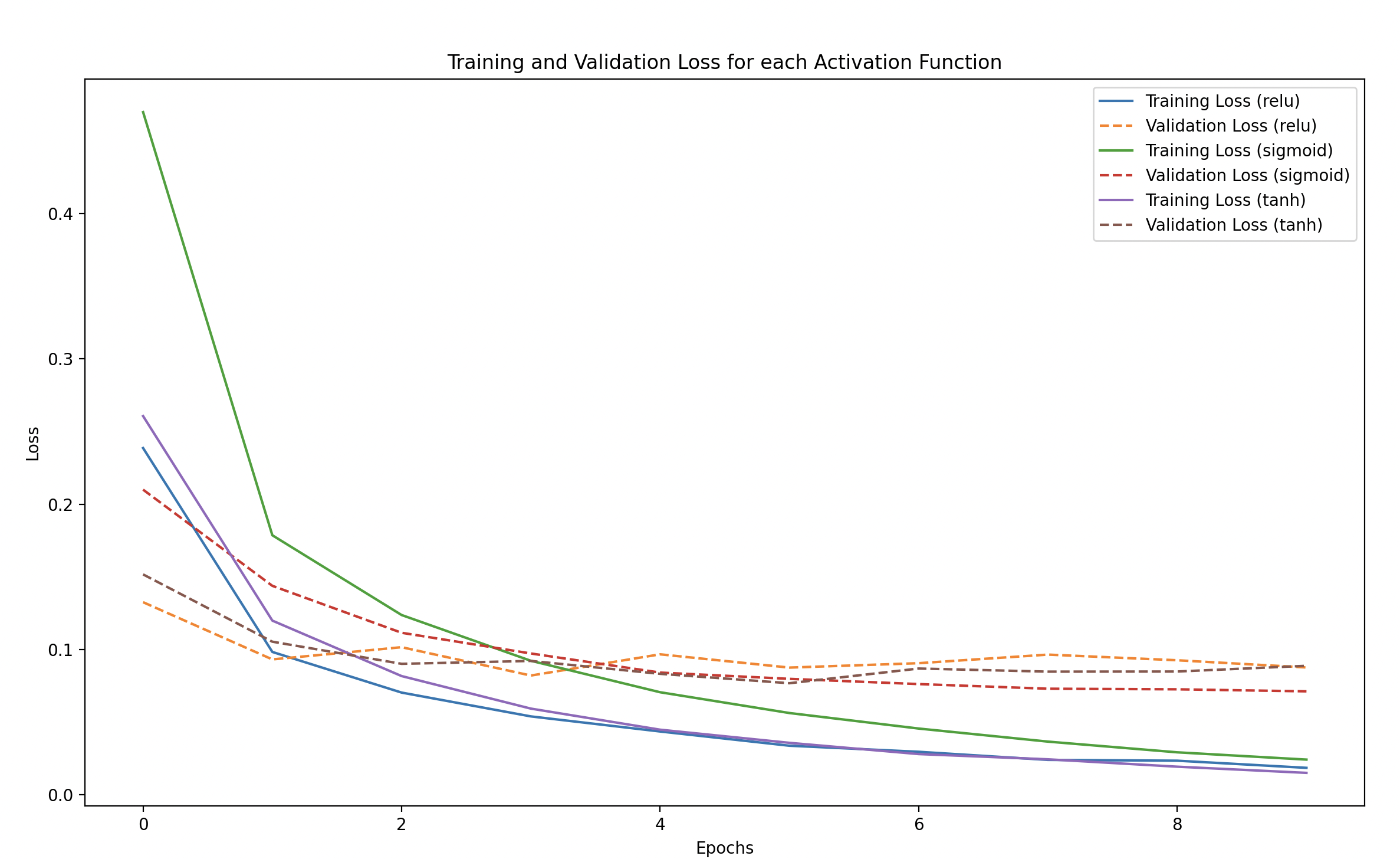
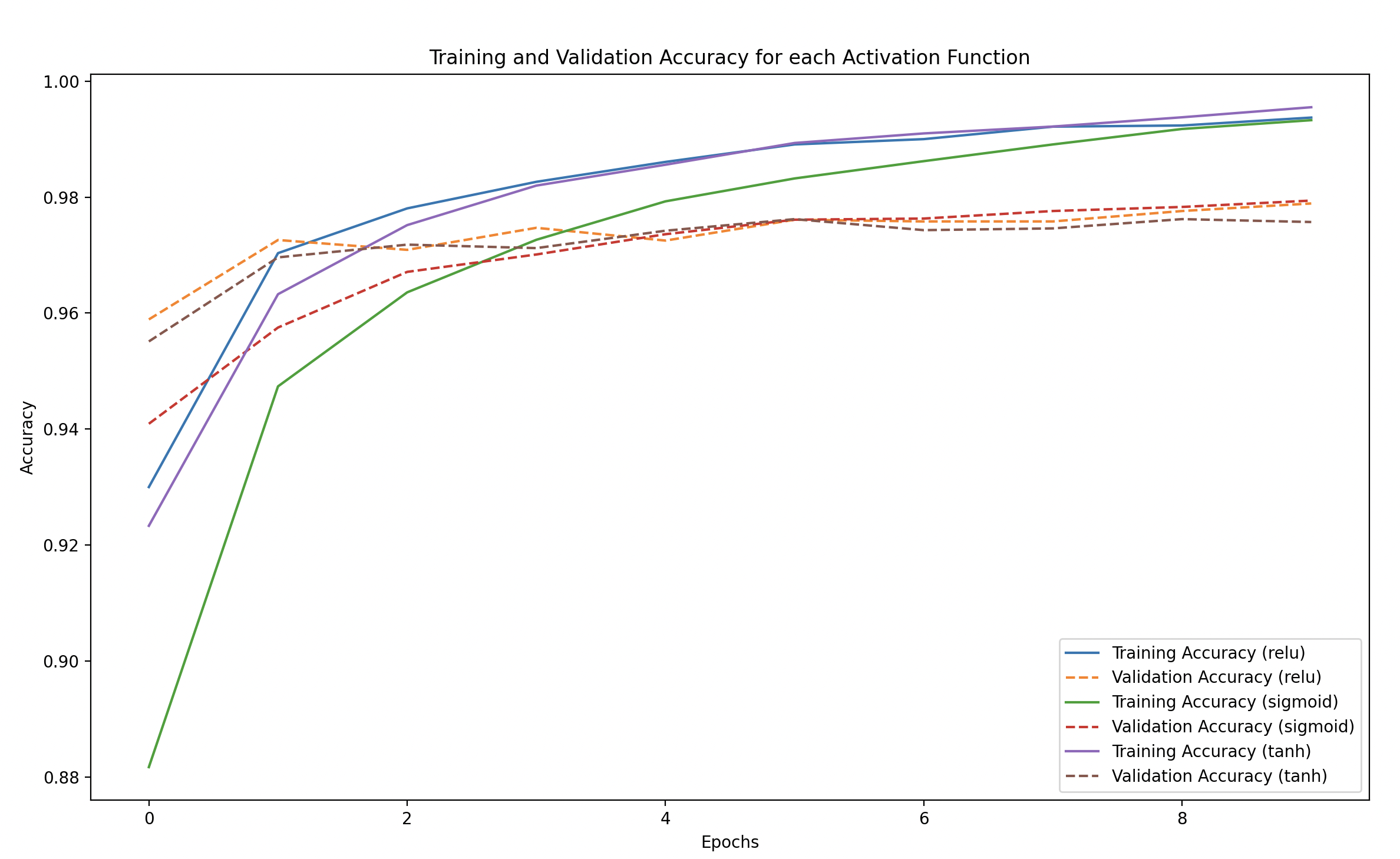
We’ll plot the training and validation accuracy as well as the loss for each activation function to compare them.
# Plot training and validation loss for each activation function
plt.figure(figsize=(14, 8))
for activation in activation_functions:
    plt.plot(history_dict[activation]['loss'], label=f'Training Loss ({activation})')
    plt.plot(history_dict[activation]['val_loss'], linestyle='--', label=f'Validation Loss ({activation})')

plt.xlabel('Epochs')
plt.ylabel('Loss')
plt.title('Training and Validation Loss for Different Activation Functions')
plt.legend()
plt.show()

# Plot training and validation accuracy for each activation function
plt.figure(figsize=(14, 8))
for activation in activation_functions:
    plt.plot(history_dict[activation]['accuracy'], label=f'Training Accuracy ({activation})')
    plt.plot(history_dict[activation]['val_accuracy'], linestyle='--', label=f'Validation Accuracy ({activation})')

plt.xlabel('Epochs')
plt.ylabel('Accuracy')
plt.title('Training and Validation Accuracy for Different Activation Functions')
plt.legend()
plt.show()
Training vs Validation Loss and Accuracy: We plot both the training and validation performance for each activation function to visually compare how well each one learns and generalizes.
What to Look for in the Results?
Training and Validation Loss
- Lower loss is better.
- Look for the speed at which the loss decreases. Faster convergence indicates that the model is learning well.
- Validation loss should be similar to training loss. If validation loss is much higher, it suggests overfitting.
Training and Validation Accuracy
- Higher accuracy is better.
- Check how quickly the model reaches a high accuracy and whether it generalizes well to the test set.
Expected Observations:
ReLU:
- Training Loss and Accuracy: ReLU is often the best for deeper networks because it doesn’t suffer from the vanishing gradient problem. It tends to converge faster and often achieves higher accuracy compared to other activations.
- Validation Performance: Usually matches training performance well, indicating good generalization.
Sigmoid:
- Training Loss and Accuracy: Sigmoid can suffer from the vanishing gradient problem, especially when there are multiple layers. This means it could learn more slowly and not reach as high an accuracy within a few epochs.
- Validation Performance: Sigmoid can sometimes overfit due to saturation, leading to poorer performance on validation data compared to ReLU or Tanh.
Tanh:
- Training Loss and Accuracy: Tanh works similarly to Sigmoid but is centered at zero, which often allows better learning dynamics because the average output is closer to zero, reducing bias in subsequent layers.
- Validation Performance: Often has better performance compared to Sigmoid but usually slower than ReLU.


Video
Coming Soon.