Day 5: Experiment With Optimizers (SGD, Adam, RMSprop) Using a Pre-Built CNN on CIFAR-10
Exploring optimizers is crucial because they control how a neural network updates its weights to minimize loss and find the best solution. For today’s task, we’ll use a pre-built Convolutional Neural Network (CNN) on the CIFAR-10 dataset and compare the impact of three popular optimizers: SGD, Adam, and RMSprop.
Overview of the Problem
- The CIFAR-10 dataset contains 60,000 color images across 10 categories (like airplanes, cars, birds, etc.).
- You will use a pre-built Convolutional Neural Network (CNN) architecture to train on this dataset.
- We’ll experiment with three optimizers:
- SGD (Stochastic Gradient Descent)
- Adam (Adaptive Moment Estimation)
- RMSprop (Root Mean Square Propagation)
Brief Overview of the Optimizers
Optimizers are like guides that help your neural network find the best solution. Imagine your neural network is a hiker trying to find the lowest point in a hilly landscape (representing the minimum loss). The optimizer is the strategy or tool the hiker uses to get to the lowest point as quickly and efficiently as possible.
Read here to know more about the optimizers.
Plan for Comparison
- Load and preprocess the CIFAR-10 dataset.
- Build a CNN model.
- Train the model using three different optimizers: SGD, Adam, and RMSprop.
- Compare the performance of each optimizer.
Let’s get started!
Step-by-Step Implementation
Step 1: Import Libraries and Load Data
import tensorflow as tf
from tensorflow.keras.datasets import cifar10
from tensorflow.keras.models import Sequential
from tensorflow.keras.layers import Conv2D, MaxPooling2D, Flatten, Dense
import matplotlib.pyplot as plt

# Load CIFAR-10 dataset
(X_train, y_train), (X_test, y_test) = cifar10.load_data()

# Normalize pixel values to between 0 and 1
X_train = X_train / 255.0
X_test = X_test / 255.0
- CIFAR-10 is a dataset of 60,000 color images (each 32x32 pixels) in 10 classes.
- Normalization of the pixel values between 0 and 1 helps improve the efficiency and stability of the training process.
Step 2: Define a Function to Build a Simple CNN Model
def build_cnn():
    model = Sequential()
    model.add(Conv2D(32, (3, 3), activation='relu', input_shape=(32, 32, 3)))
    model.add(MaxPooling2D((2, 2)))
    model.add(Conv2D(64, (3, 3), activation='relu'))
    model.add(MaxPooling2D((2, 2)))
    model.add(Conv2D(64, (3, 3), activation='relu'))
    model.add(Flatten())
    model.add(Dense(64, activation='relu'))
    model.add(Dense(10, activation='softmax'))
    return model
- We define a function build_cnn() that returns a simple CNN model.
- Conv2D layers with ReLU activation extract features from images.
- MaxPooling2D reduces the dimensions of the feature maps.
- The final layers are fully connected (Dense) layers, ending with softmax to output 10 classes.
Step 3: Train the Model with Different Optimizers
We will train the model using SGD, Adam, and RMSprop and compare their performance.
# List of optimizers to compare
optimizers = {
    'SGD': tf.keras.optimizers.SGD(learning_rate=0.01, momentum=0.9),
    'Adam': tf.keras.optimizers.Adam(learning_rate=0.001),
    'RMSprop': tf.keras.optimizers.RMSprop(learning_rate=0.001)
}

# Dictionary to store the training history of each optimizer
history_dict = {}

for opt_name, opt in optimizers.items():
    # Build and compile the model with a specific optimizer
    model = build_cnn()
    model.compile(optimizer=opt,
                  loss='sparse_categorical_crossentropy',
                  metrics=['accuracy'])

    # Train the model
    print(f"Training with optimizer: {opt_name}")
    history = model.fit(X_train, y_train,
                        validation_data=(X_test, y_test),
                        epochs=10,
                        batch_size=64,
                        verbose=1)

    # Store the history for comparison
    history_dict[opt_name] = history.history
Optimizers:
SGD(learning_rate=0.01, momentum=0.9): Includes momentum to make the updates smoother and potentially faster.Adam(learning_rate=0.001): Uses adaptive learning rates, popular for most use-cases.RMSprop(learning_rate=0.001): Also uses adaptive learning rates to stabilize training.
Model Compilation and Training:
- Each model is compiled with a specific optimizer.
epochs=10: We train each model for 10 epochs to get an initial comparison.
Step 4: Visualize and Compare the Results
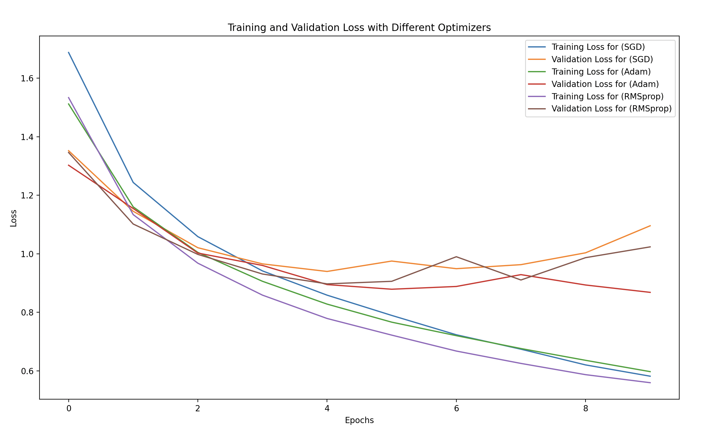
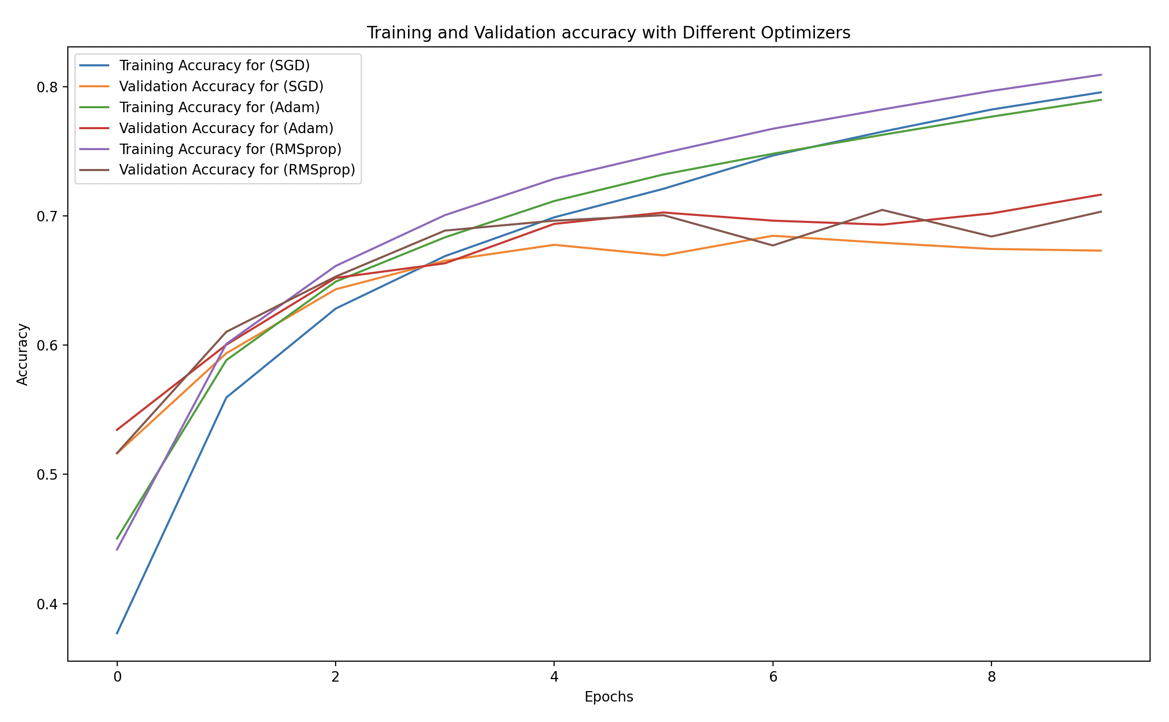
We will plot the training and validation accuracy and loss for each optimizer to compare their effectiveness.
# Plot training and validation loss for each optimizer
plt.figure(figsize=(14, 8))
for opt_name in optimizers.keys():
    plt.plot(history_dict[opt_name]['loss'], label=f'Training Loss ({opt_name})')
    plt.plot(history_dict[opt_name]['val_loss'], linestyle='--', label=f'Validation Loss ({opt_name})')

plt.xlabel('Epochs')
plt.ylabel('Loss')
plt.title('Training and Validation Loss for Different Optimizers')
plt.legend()
plt.show()

# Plot training and validation accuracy for each optimizer
plt.figure(figsize=(14, 8))
for opt_name in optimizers.keys():
    plt.plot(history_dict[opt_name]['accuracy'], label=f'Training Accuracy ({opt_name})')
    plt.plot(history_dict[opt_name]['val_accuracy'], linestyle='--', label=f'Validation Accuracy ({opt_name})')

plt.xlabel('Epochs')
plt.ylabel('Accuracy')
plt.title('Training and Validation Accuracy for Different Optimizers')
plt.legend()
plt.show()
- Training vs Validation Loss and Accuracy:
- We plot both the training and validation performance for each optimizer.
- This will help you visually understand how well each optimizer performs in terms of both learning speed and generalization.
What to Look for in the Results?
Training and Validation Loss
- Lower loss is better.
- Look for the speed at which the loss decreases. Faster convergence indicates that the model is learning well.
- Validation loss should be similar to training loss. If validation loss is much higher, it suggests overfitting.
Training and Validation Accuracy
- Higher accuracy is better.
- Check how quickly the model reaches a high accuracy and whether it generalizes well to the test set.
Expected Observations
SGD:
- Training Loss and Accuracy: May take longer to converge, and the loss might not decrease as steadily.
- Validation Performance: Often less stable than adaptive optimizers, but with enough epochs, it can catch up.
Adam:
- Training Loss and Accuracy: Expected to have faster convergence and stable learning. You should see the loss decreasing quickly, and accuracy improving steadily.
- Validation Performance: Usually good, with high validation accuracy that is close to training accuracy, suggesting good generalization.
RMSprop:
- Training Loss and Accuracy: Similar to Adam, RMSprop often works well with adaptive learning rates and can converge quickly.
- Validation Performance: Typically shows a steady improvement, often comparable to Adam.

