Day 6: Apply dropout and regularization (L2) for overfitting control (Titanic Dataset)

Today, we’ll explore two key techniques for controlling overfitting: Dropout and L2 Regularization. We’ll apply these techniques to a model trained on the Titanic dataset, which is a well-known dataset containing information about passengers, like their age, gender, ticket class, etc., with the goal of predicting survival.

What is Overfitting?

#

• Overfitting occurs when a model learns the training data too well, including its noise and irrelevant details, and fails to generalize to new, unseen data.
• It’s like a student who memorizes every page of a book instead of understanding the main concepts — they might do well in a test with the exact same questions but will struggle when the questions are different.

Two techniques to prevent overfitting are Dropout and L2 Regularization.

What is Dropout?

#

• Dropout is a technique where, during training, we randomly turn off some neurons in the network.
• In simple terms, dropout forces the network to learn more robust features instead of relying on just a few neurons to make predictions.

What is L2 Regularization?

#

• L2 Regularization is a technique where we penalize large weights in the neural network.
• The idea is to keep the weights small so that the model doesn’t rely too heavily on any particular feature.

Plan:

#

• Load the Titanic dataset and preprocess it.
• Build a neural network and apply Dropout and L2 Regularization.
• Train the model and observe the effect on overfitting.

Step-by-Step Implementation

#

Step 1: Import Libraries and Load Data

#

First, we’ll import the necessary libraries and load the Titanic dataset using Pandas.

import pandas as pd
import numpy as np
import tensorflow as tf
from sklearn.model_selection import train_test_split
from sklearn.preprocessing import StandardScaler
from tensorflow.keras.models import Sequential
from tensorflow.keras.layers import Dense, Dropout
from tensorflow.keras.regularizers import l2

# Load Titanic dataset from seaborn (for simplicity)
import seaborn as sns
titanic = sns.load_dataset('titanic')

# Display the first few rows to understand the structure
print(titanic.head())

• We’re using Seaborn to load the Titanic dataset for simplicity. You could use Pandas to load the dataset from a CSV as well.
• Display the first few rows to get an understanding of the data structure.

Step 2: Preprocess the Data

#

We’ll need to preprocess the dataset:

• Remove unnecessary columns.
• Fill missing values.
• Convert categorical columns to numerical.

# Drop columns that are not useful for prediction
titanic = titanic.drop(['embarked', 'class', 'who', 'adult_male', 'alive', 'deck', 'embark_town', 'sex'], axis=1)

# Fill missing values
titanic['age'].fillna(titanic['age'].mean(), inplace=True)
titanic['fare'].fillna(titanic['fare'].mean(), inplace=True)

# Convert categorical columns to numerical
titanic['embarked'] = titanic['embarked'].astype('category').cat.codes
titanic['sex'] = titanic['sex'].astype('category').cat.codes

# Split the dataset into features and labels
X = titanic.drop('survived', axis=1)
y = titanic['survived']

# Split into training and testing sets
X_train, X_test, y_train, y_test = train_test_split(X, y, test_size=0.2, random_state=42)

# Standardize the data
scaler = StandardScaler()
X_train = scaler.fit_transform(X_train)
X_test = scaler.transform(X_test)

• Drop unnecessary columns: Columns like who, embark_town, sex are either redundant or not useful for training.
• Fill missing values: Filling missing values in age and fare helps maintain data consistency.
• Convert categorical columns: Convert categorical features (like sex) into numerical codes.
• Standardize the data: Scaling the features helps in faster and more efficient training.

Step 3: Build the Model with Dropout and L2 Regularization

#

Next, we’ll build a neural network model with L2 Regularization and Dropout layers.

# Build the neural network model with Dropout and L2 Regularization
model = Sequential()
model.add(Dense(128, activation='relu', input_shape=(X_train.shape[1],), kernel_regularizer=l2(0.01)))
model.add(Dropout(0.5))  # Dropout rate of 50%
model.add(Dense(64, activation='relu', kernel_regularizer=l2(0.01)))
model.add(Dropout(0.3))  # Dropout rate of 30%
model.add(Dense(1, activation='sigmoid'))

# Compile the model
model.compile(optimizer='adam', loss='binary_crossentropy', metrics=['accuracy'])

# Display the model summary
model.summary()

• Dense(128, activation=‘relu’, kernel_regularizer=l2(0.01)): Adds a hidden layer with 128 neurons and L2 regularization. The L2 penalty (0.01) helps keep weights from growing too large.
• Dropout(0.5): Randomly drops 50% of neurons in this layer during training. This prevents the model from being overly reliant on any specific neurons.
• The output layer is a single neuron with a sigmoid activation function, used for binary classification.

Step 4: Train the Model

#

Now, we will train the model and observe how it performs over the epochs.

# Train the model
history = model.fit(X_train, y_train, validation_data=(X_test, y_test), epochs=50, batch_size=32, verbose=1)

# Convert the history to a DataFrame for easy viewing
history_df = pd.DataFrame(history.history)

# Display the first few rows of the training history DataFrame
print(history_df.head())

• model.fit(): Trains the model on the training data for 50 epochs with a batch size of 32.
• We convert the training history to a Pandas DataFrame to make it easy to visualize the training and validation performance.

Step 5: Visualize Training and Validation Performance

#

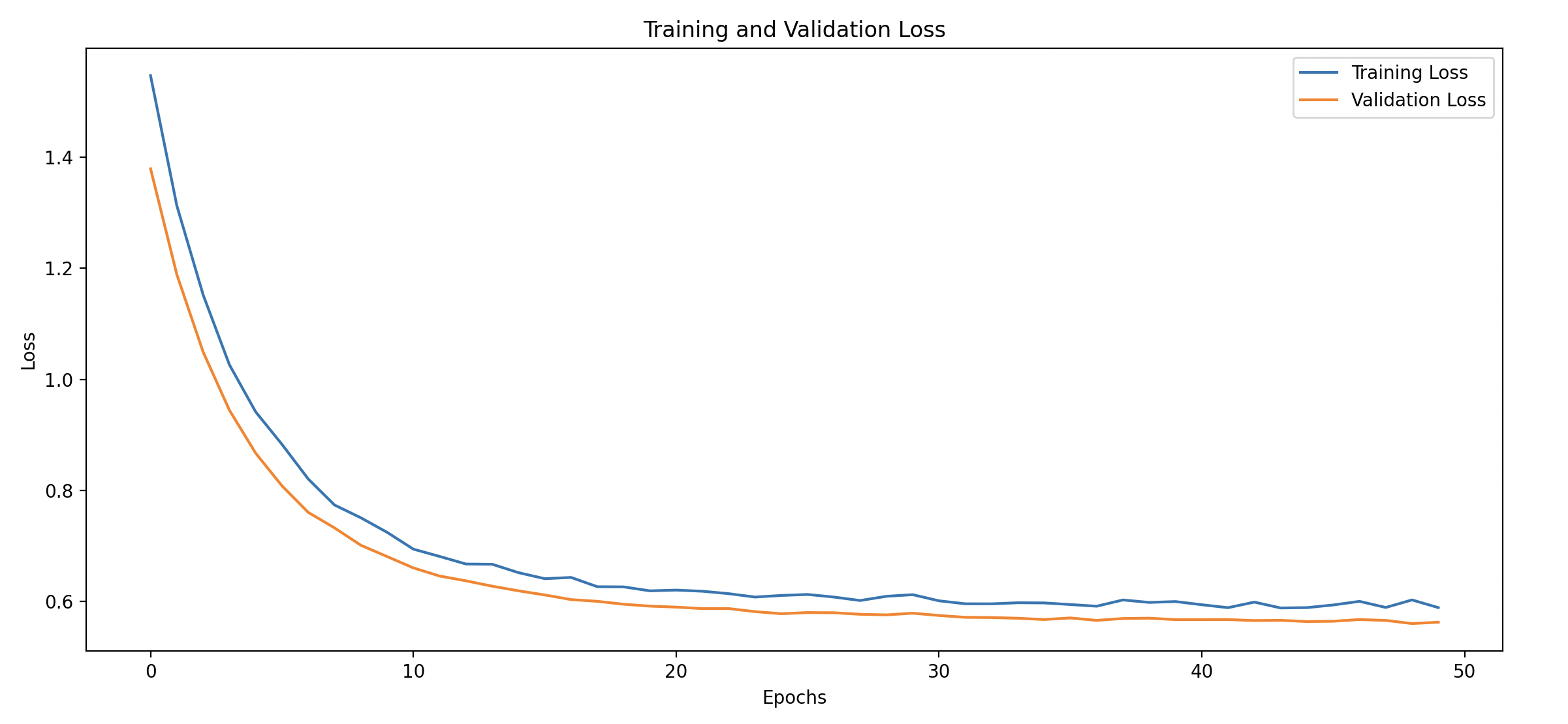
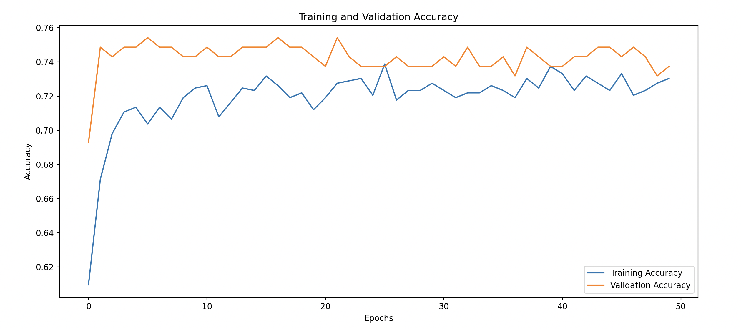
We will plot the training and validation loss and accuracy to see how well the model is controlling overfitting.

import matplotlib.pyplot as plt

# Plot training and validation loss
plt.figure(figsize=(14, 6))
plt.plot(history_df['loss'], label='Training Loss')
plt.plot(history_df['val_loss'], label='Validation Loss', linestyle='--')
plt.xlabel('Epochs')
plt.ylabel('Loss')
plt.title('Training and Validation Loss')
plt.legend()
plt.show()

# Plot training and validation accuracy
plt.figure(figsize=(14, 6))
plt.plot(history_df['accuracy'], label='Training Accuracy')
plt.plot(history_df['val_accuracy'], label='Validation Accuracy', linestyle='--')
plt.xlabel('Epochs')
plt.ylabel('Accuracy')
plt.title('Training and Validation Accuracy')
plt.legend()
plt.show()

• Training vs Validation Loss: Look for differences between the training and validation loss. A significant gap could indicate overfitting.
• Training vs Validation Accuracy: A good model will have training and validation accuracies that are close to each other, showing that it generalizes well.

Video

#