Day 8: Build a Simple CNN for CIFAR-10 Image Classification
- Today, we will build a simple CNN for image classification on the CIFAR-10 dataset.
- The CIFAR-10 dataset contains 60,000 color images of size 32x32 pixels, with 10 categories like airplanes, birds, cars, etc.
- We’ll use TensorFlow and Keras to build and train a Convolutional Neural Network (CNN), which is well-suited for handling image data due to its unique ability to capture spatial relationships in the data.
What is a Convolutional Neural Network (CNN)?
A Convolutional Neural Network (CNN) is a type of deep learning model specially designed to work with images. CNNs can recognize patterns in images, much like how we use our eyes and brain to recognize faces, objects, and everything around us.
Think of a CNN as a series of layers that each work together to identify features in an image, much like how our brain processes visual information step by step.
Imagine a Simple Example: Recognizing a Cat Picture
Imagine you’re looking at a picture of a cat. How do you know it’s a cat? Well, your brain processes the picture in parts. You might notice the whiskers, the eyes, the ears, and the shape of the face. Similarly, a CNN looks at the picture and breaks it down into parts to decide if it’s a cat.
How CNNs Work:
A CNN is composed of a series of layers, each working as a specialist to examine different parts of the image, each time getting more detailed. Here’s how it works (with cat example):
- Input Image: A picture of a cat is given to the CNN.
- Convolution Layer: The CNN applies filters to detect basic features, like edges or colors.
- Pooling Layer: The network simplifies the image, keeping only the essential information.
- Flattening: It turns the pooled image into a list of key features.
- Fully Connected Layer: The CNN examines the list of features and decides if it’s a cat, dog, bird, or something else.

Read more for in depth understanding, with easy examples.
Step-by-Step Guide to Build a Simple CNN for CIFAR-10
Step 1: Import Necessary Libraries
We start by importing TensorFlow, Keras, and other helpful libraries.
import tensorflow as tf
from tensorflow.keras.models import Sequential
from tensorflow.keras.layers import Conv2D, MaxPooling2D, Flatten, Dense
from tensorflow.keras.layers import Dropout
from tensorflow.keras.datasets import cifar10
from tensorflow.keras.utils import to_categorical
import matplotlib.pyplot as plt
Explanation:
- TensorFlow and Keras help us easily build and train the CNN.
Conv2D,MaxPooling2D,Dropout,Flatten,Denseare layers used to build our CNN.cifar10is the dataset we will work with.
Step 2: Load and Preprocess the CIFAR-10 Dataset
We’ll load the CIFAR-10 dataset and prepare it for training.
# Load CIFAR-10 dataset
(X_train, y_train), (X_test, y_test) = cifar10.load_data()

# Normalize pixel values to be between 0 and 1
X_train = X_train.astype('float32') / 255.0
X_test = X_test.astype('float32') / 255.0

# Convert labels to categorical format (One-hot encoding)
y_train = to_categorical(y_train, 10)
y_test = to_categorical(y_test, 10)
Explanation:
- Load Data: CIFAR-10 is already split into training and test sets.
X_traincontains the image data, andy_traincontains the labels. - Normalization: Pixel values are scaled between 0 and 1 to improve training.
- One-hot Encoding: Converts labels to one-hot format, needed for multi-class classification.
Step 3: Define the CNN Model
We’ll build a simple CNN with two convolutional layers followed by fully connected layers for classification.
# Define the CNN model
model = Sequential()

# First Convolutional Layer
model.add(Conv2D(32, (3, 3), activation='relu', input_shape=(32, 32, 3)))
model.add(MaxPooling2D((2, 2)))

# Second Convolutional Layer
model.add(Conv2D(64, (3, 3), activation='relu'))
model.add(MaxPooling2D((2, 2)))

# Flatten the output to feed into fully connected layers
model.add(Flatten())

# Fully Connected Layer
model.add(Dense(64, activation='relu'))

# Dropout Layer to avoid overfitting
model.add(Dropout(0.5))

# Output Layer
model.add(Dense(10, activation='softmax'))

# Compile the model
model.compile(optimizer='adam', loss='categorical_crossentropy', metrics=['accuracy'])

# Summary of the model
model.summary()
Explanation:
- Conv2D(32, (3, 3), activation=‘relu’, input_shape=(32, 32, 3)): Applies 32 filters of size 3x3 with ReLU activation. The input shape is set to (32, 32, 3) for CIFAR-10 images.
- MaxPooling2D((2, 2)): Reduces spatial dimensions by taking the maximum value from each 2x2 region.
- Flatten(): Flattens 2D feature maps into a 1D vector for the fully connected layer.
- Dense(64, activation=‘relu’): Adds a fully connected layer with 64 neurons.
- Dropout(0.5): Randomly drops 50% of neurons during training to prevent overfitting.
- Dense(10, activation=‘softmax’): Output layer with 10 neurons for CIFAR-10 classes, using softmax for probability distribution.
- model.compile(): The model is compiled with the Adam optimizer, categorical cross-entropy loss, and accuracy as the metric.
Step 4: Train the Model
Now, we’ll train the model on the CIFAR-10 dataset.
# Train the model
history = model.fit(X_train, y_train, epochs=20, batch_size=32, validation_data=(X_test, y_test), verbose=1)
Explanation:
- epochs=20: The model trains for 20 epochs over the dataset.
- batch_size=32: 32 samples per gradient update.
- validation_data=(X_test, y_test): Enables evaluation on unseen data during training.
Step 5: Evaluate the Model
We’ll evaluate the model on the test data to assess its performance.
# Evaluate the model on the test set
test_loss, test_accuracy = model.evaluate(X_test, y_test, verbose=2)
print(f'Test accuracy: {test_accuracy:.2f}')
Explanation:
- model.evaluate(): Calculates the loss and accuracy on the test set.
- test_accuracy: Provides an estimate of how well the model generalizes to unseen data.
Step 6: Visualize Training Performance
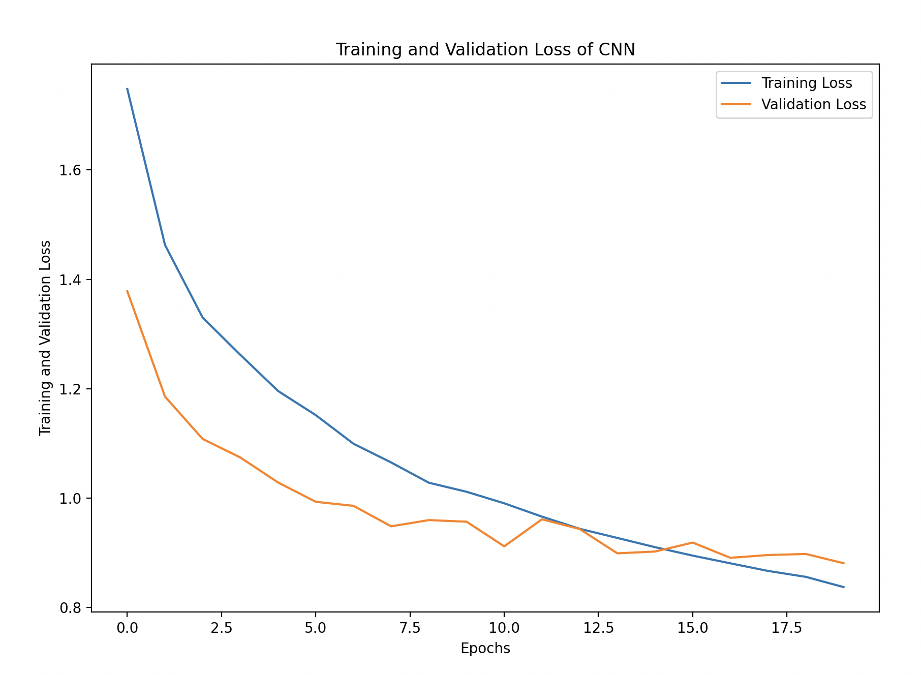
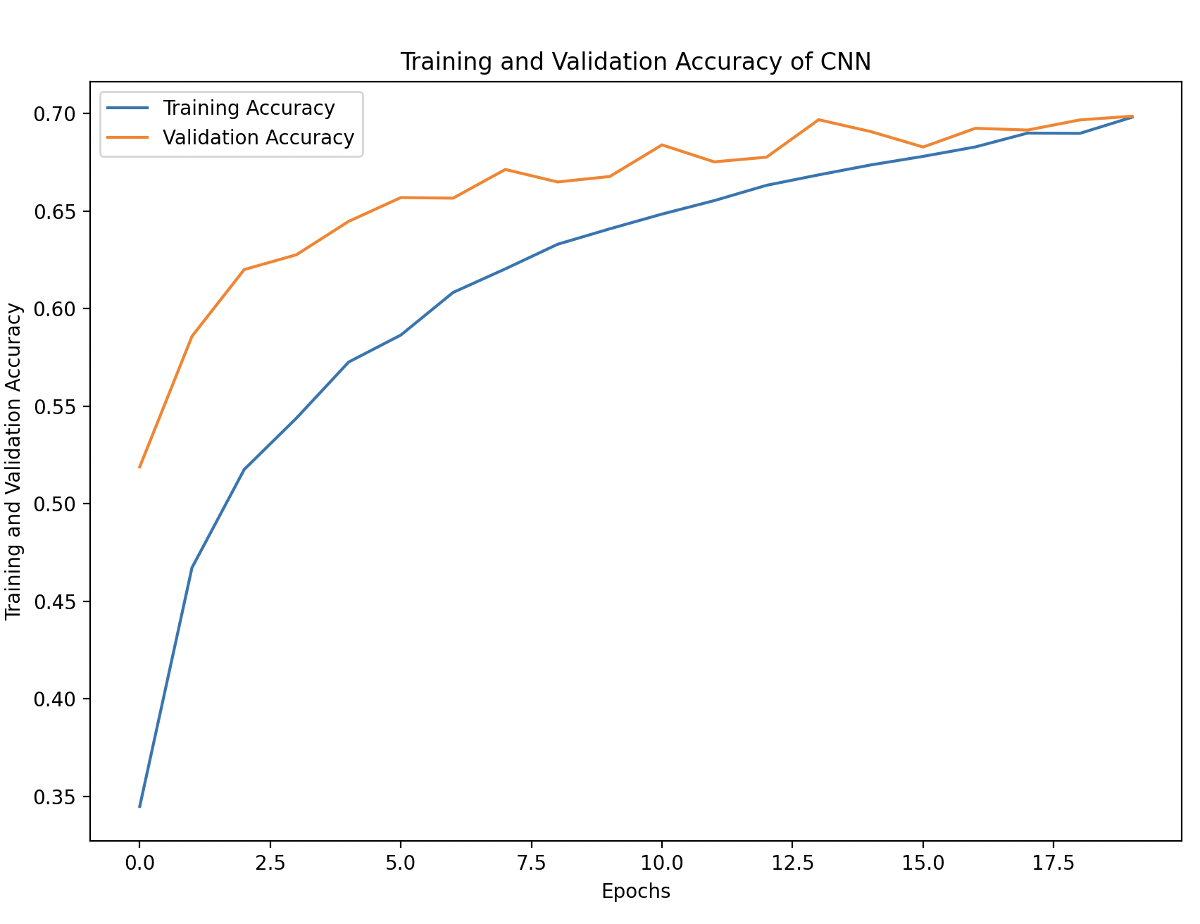
We can plot the training history to observe the model’s learning process over time.
# Convert the history to a DataFrame for easy visualization
import pandas as pd
history_df = pd.DataFrame(history.history)

# Plot training and validation accuracy
plt.figure(figsize=(10, 6))
plt.plot(history_df['accuracy'], label='Training Accuracy')
plt.plot(history_df['val_accuracy'], linestyle='--', label='Validation Accuracy')
plt.xlabel('Epochs')
plt.ylabel('Accuracy')
plt.title('Training and Validation Accuracy')
plt.legend()
plt.show()

# Plot training and validation loss
plt.figure(figsize=(10, 6))
plt.plot(history_df['loss'], label='Training Loss')
plt.plot(history_df['val_loss'], linestyle='--', label='Validation Loss')
plt.xlabel('Epochs')
plt.ylabel('Loss')
plt.title('Training and Validation Loss')
plt.legend()
plt.show()
Explanation:
- history_df[‘accuracy’] and history_df[‘val_accuracy’]: Shows how the model performs on the training and validation set over time.
- Training and Validation Loss: Helps identify if the model is overfitting by comparing training and validation loss.

