Day 22: GAN Basics - Understanding GAN Architecture and Setting Up a GAN Framework

Today, we explored the basics of Generative Adversarial Networks (GANs). GANs are one of the most innovative approaches in deep learning, used for generating data that closely resembles the training dataset. They have gained popularity in various fields, including art, image generation, and even data augmentation for machine learning models. In today’s session, we set up a basic GAN framework using the Fashion MNIST dataset.

Step 1: Understanding GAN Architecture

A Generative Adversarial Network (GAN) consists of two neural networks that compete with each other:

Generator: This network generates synthetic data that should look like the real data. For Fashion MNIST, it generates synthetic images of clothing items.
Discriminator: This network evaluates the authenticity of data, distinguishing between real and fake images. It classifies whether the input is a real image from the dataset or a fake image produced by the generator.

These two models are trained in a competitive fashion, where:

The Generator tries to fool the Discriminator by creating realistic-looking data.
The Discriminator tries to accurately identify whether the data is real or fake.

This competition helps both models improve simultaneously in what is called adversarial training.

Step 2: Import Libraries and Load Dataset

First, we import the necessary libraries and load the Fashion MNIST dataset, which is a collection of grayscale images of clothing items.

import numpy as np
import tensorflow as tf
from tensorflow.keras.layers import Dense, Flatten, Reshape, LeakyReLU, BatchNormalization
from tensorflow.keras.models import Sequential
import matplotlib.pyplot as plt

TensorFlow/Keras: Used for building the generator and discriminator models.
NumPy: Helps in handling data efficiently.
Matplotlib: Used to visualize the generated images.

Load the dataset:

# Load Fashion MNIST dataset
(X_train, _), (_, _) = tf.keras.datasets.fashion_mnist.load_data()

# Normalize the images between -1 and 1
X_train = (X_train - 127.5) / 127.5
X_train = X_train.reshape(X_train.shape[0], 28, 28, 1).astype('float32')

Normalization: We normalize the data to have values between -1 and 1 to match the output range of the tanh activation function used in the generator.
Reshape: We reshape the images to 28x28x1 to explicitly define them as grayscale images.

Step 3: Build the Generator

The Generator takes random noise and generates synthetic images that resemble real Fashion MNIST images (28x28).

# Define the Generator
def build_generator():
    model = Sequential()

    # Dense layer to increase dimensionality from noise
    model.add(Dense(256, input_dim=100))
    model.add(LeakyReLU(alpha=0.2))
    model.add(BatchNormalization(momentum=0.8))

    # Another Dense layer
    model.add(Dense(512))
    model.add(LeakyReLU(alpha=0.2))
    model.add(BatchNormalization(momentum=0.8))

    # One more Dense layer
    model.add(Dense(1024))
    model.add(LeakyReLU(alpha=0.2))
    model.add(BatchNormalization(momentum=0.8))

    # Final output layer, reshaping to 28x28x1
    model.add(Dense(28 * 28 * 1, activation='tanh'))
    model.add(Reshape((28, 28, 1)))

    return model

generator = build_generator()
generator.summary()

Dense Layers: The generator uses several dense layers to upscale a random noise vector (size 100) into an image-sized output (28x28x1).
LeakyReLU Activation: LeakyReLU helps to avoid dead neurons by allowing a small gradient for negative inputs (alpha=0.2).
BatchNormalization: Helps stabilize training and improves convergence speed.
Output Layer: The final layer uses tanh activation, ensuring output pixel values are between -1 and 1.

Step 4: Build the Discriminator

The Discriminator takes an image and outputs whether it believes the image is real or fake.

# Define the Discriminator
def build_discriminator():
    model = Sequential()

    # Flatten the input image
    model.add(Flatten(input_shape=(28, 28, 1)))

    # Dense layer to process the flattened image
    model.add(Dense(512))
    model.add(LeakyReLU(alpha=0.2))

    # Another Dense layer
    model.add(Dense(256))
    model.add(LeakyReLU(alpha=0.2))

    # Final output layer to classify real or fake
    model.add(Dense(1, activation='sigmoid'))

    return model

discriminator = build_discriminator()
discriminator.compile(optimizer='adam', loss='binary_crossentropy', metrics=['accuracy'])
discriminator.summary()

Dense Layers: Uses dense layers to analyze the input.
LeakyReLU: Similar to the generator, LeakyReLU is used to allow non-zero gradients for negative values.
Output Layer: Uses sigmoid activation to output a value between 0 (fake) and 1 (real).
Binary Crossentropy Loss: Suitable for a binary classification problem (real vs fake).

Step 5: Build and Compile the GAN

Now, let’s build and compile the GAN by combining the Generator and Discriminator.

# Freeze the Discriminator's weights during GAN training
discriminator.trainable = False

# Build and compile the GAN
def build_gan(generator, discriminator):
    model = Sequential()
    model.add(generator)
    model.add(discriminator)
    return model

gan = build_gan(generator, discriminator)
gan.compile(optimizer='adam', loss='binary_crossentropy')

Freeze Discriminator: We freeze the discriminator’s weights while training the GAN so that the discriminator doesn’t get updated when training the generator.
GAN Model: Combines the generator and discriminator so that the generator can be trained to fool the discriminator.

Step 6: Training the GAN

The training loop involves iteratively training the discriminator and then the generator.

# Training parameters
epochs = 10000
batch_size = 64
save_interval = 1000

# Labels for real and fake images
real = np.ones((batch_size, 1))
fake = np.zeros((batch_size, 1))

for epoch in range(epochs):
    # Train the Discriminator
    idx = np.random.randint(0, X_train.shape[0], batch_size)
    real_images = X_train[idx]

    noise = np.random.normal(0, 1, (batch_size, 100))
    generated_images = generator.predict(noise)

    d_loss_real = discriminator.train_on_batch(real_images, real)
    d_loss_fake = discriminator.train_on_batch(generated_images, fake)
    d_loss = 0.5 * np.add(d_loss_real, d_loss_fake)

    # Train the Generator
    noise = np.random.normal(0, 1, (batch_size, 100))
    g_loss = gan.train_on_batch(noise, real)

    # Print progress
    if epoch % save_interval == 0:
        print(f"{epoch} [D loss: {d_loss[0]}, acc.: {100 * d_loss[1]}%] [G loss: {g_loss}]")

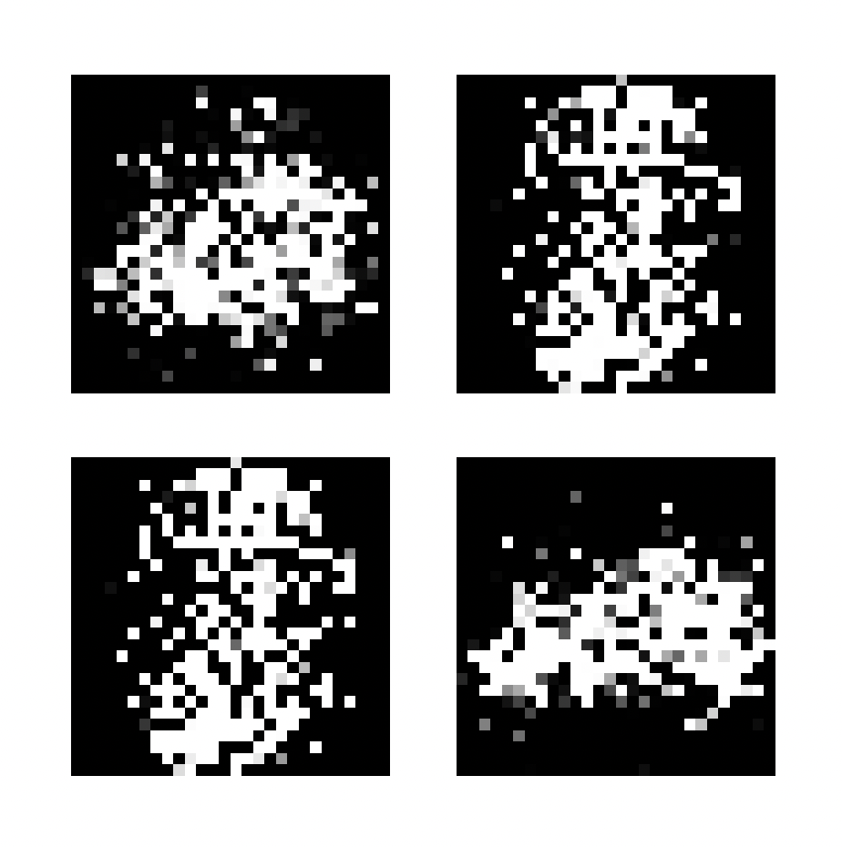
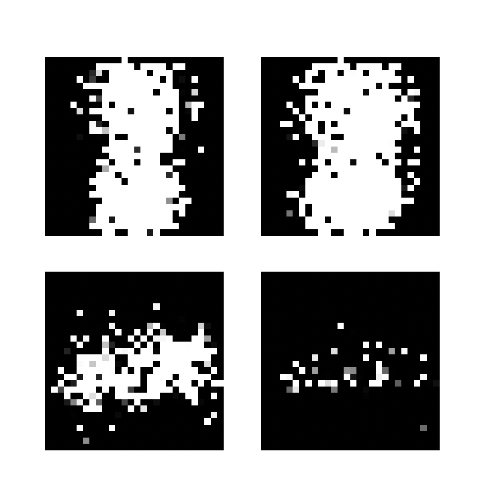
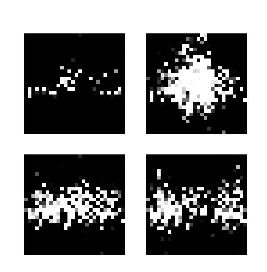
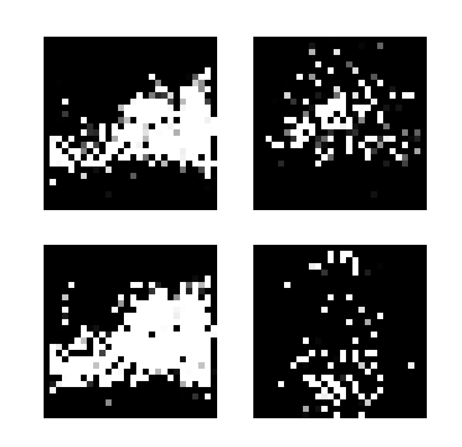
        # Save generated images to visualize training progress
        generated_images = generator.predict(noise)
        generated_images = 0.5 * generated_images + 0.5  # Rescale images from -1 to 1 to 0 to 1

        plt.figure(figsize=(5, 5))
        for i in range(4):
            plt.subplot(2, 2, i + 1)
            plt.imshow(generated_images[i, :, :, 0], cmap='gray')
            plt.axis('off')
        plt.show()

Discriminator Training: We train the discriminator on a mix of real and fake images.
Generator Training: The generator is trained via the GAN model to try and fool the discriminator.
Save Interval: Every 1000 epochs, generated images are saved to monitor training progress.

Summary of Performance

Initial Outputs: The initial outputs of the generator were blurry and noisy, which is expected in early epochs.
Discriminator vs Generator Balance: The discriminator is often too good at the start, making it hard for the generator to improve. This leads to noisy and meaningless generated images.

Some generated images: