Day 11 - 30 Days 30 Machine Learning Projects: Anomaly Detection With Isolation Forest
The Problem
On Day 11 of the 30 Day 30 Machine Learning Projects Challenge, we focused on detecting credit card fraud using an Isolation Forest model. The goal was to identify anomalies in transaction data, labeling these anomalies as potential fraud cases.
If you want to see the code, you can find it here: GIT REPO.
Understanding the Data
We used the Credit Card Fraud Detection Dataset from Kaggle. The dataset includes transactions labeled as either normal (0) or fraud (1). In this project, we used Isolation Forest to separate the normal and fraudulent transactions.
Code Workflow
The steps involved were as follows:
- Load the Data
- Create Feature and Target datasets
- Split the Data
- Build and Train the Model
- Make Predictions and Evaluate
- Visualization
Step 1: Load the data
Download the data from kaggle and put it in the dataset directory at the root of your project.
data = pd.read_csv('dataset/creditcard.csv')
Step 2: Create Feature and Target Datasets
We separated the features (X) and target labels (y). Additionally, we mapped the target labels for consistency with the Isolation Forest model, where 1 represents normal transactions and -1 represents fraud (anomalies).
X = data.drop('Class', axis=1)
y = data['Class'].map({0: 1, 1: -1})  # 1: Normal, -1: Fraud/Anomaly
Step 3: Split the Data
We split the dataset into 80% training and 20% validation sets. To ensure the distribution of normal and fraud transactions remains balanced across the training and validation sets, we used stratification:
X_train, X_val, y_train, y_val = train_test_split(X, y, test_size=0.2, random_state=42, stratify=y)
Step 4: Build and Train the Isolation Forest Model
We used Isolation Forest, which is an unsupervised algorithm for anomaly detection. The contamination parameter was set to 0.01 (assuming 1% of the data are anomalies).
model = IsolationForest(contamination=0.01, random_state=42)
model.fit(X_train)
Step 5: Make Predictions and Evaluate
The model predicted whether each transaction was normal (1) or an anomaly (-1). We used a confusion matrix and other metrics to evaluate the model’s performance.
predictions = model.predict(X_val)
X_val['anomaly'] = predictions

accuracy = accuracy_score(y_val, predictions)
conf_matrix = confusion_matrix(y_val, predictions)
class_report = classification_report(y_val, predictions, zero_division=1)

print(f"Accuracy Score: {accuracy}")
print(f"Confusion Matrix:\n{conf_matrix}")
print(f"Classification Report:\n{class_report}")
Key Metrics:
- True Positives (fraud correctly identified as fraud)
- False Positives (normal transactions mistakenly flagged as fraud)
- False Negatives (fraud missed by the model)
- True Negatives (normal transactions correctly identified)
Step 6: Visualization
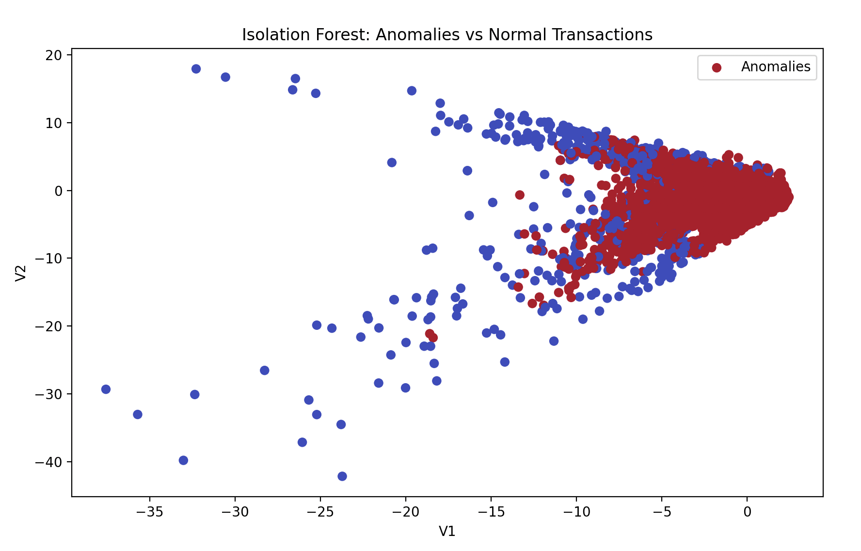
We created a scatter plot to visualize the anomalies versus normal transactions based on two features (V1 and V2), and used a confusion matrix heatmap to show the model’s performance.
Scatter Plot:
plt.figure(figsize=(10, 6))
plt.scatter(X_val['V1'], X_val['V2'], c=predictions, cmap='coolwarm', label='Anomalies')
plt.xlabel('V1')
plt.ylabel('V2')
plt.title('Isolation Forest: Anomalies vs Normal Transactions')
plt.legend()
plt.show()
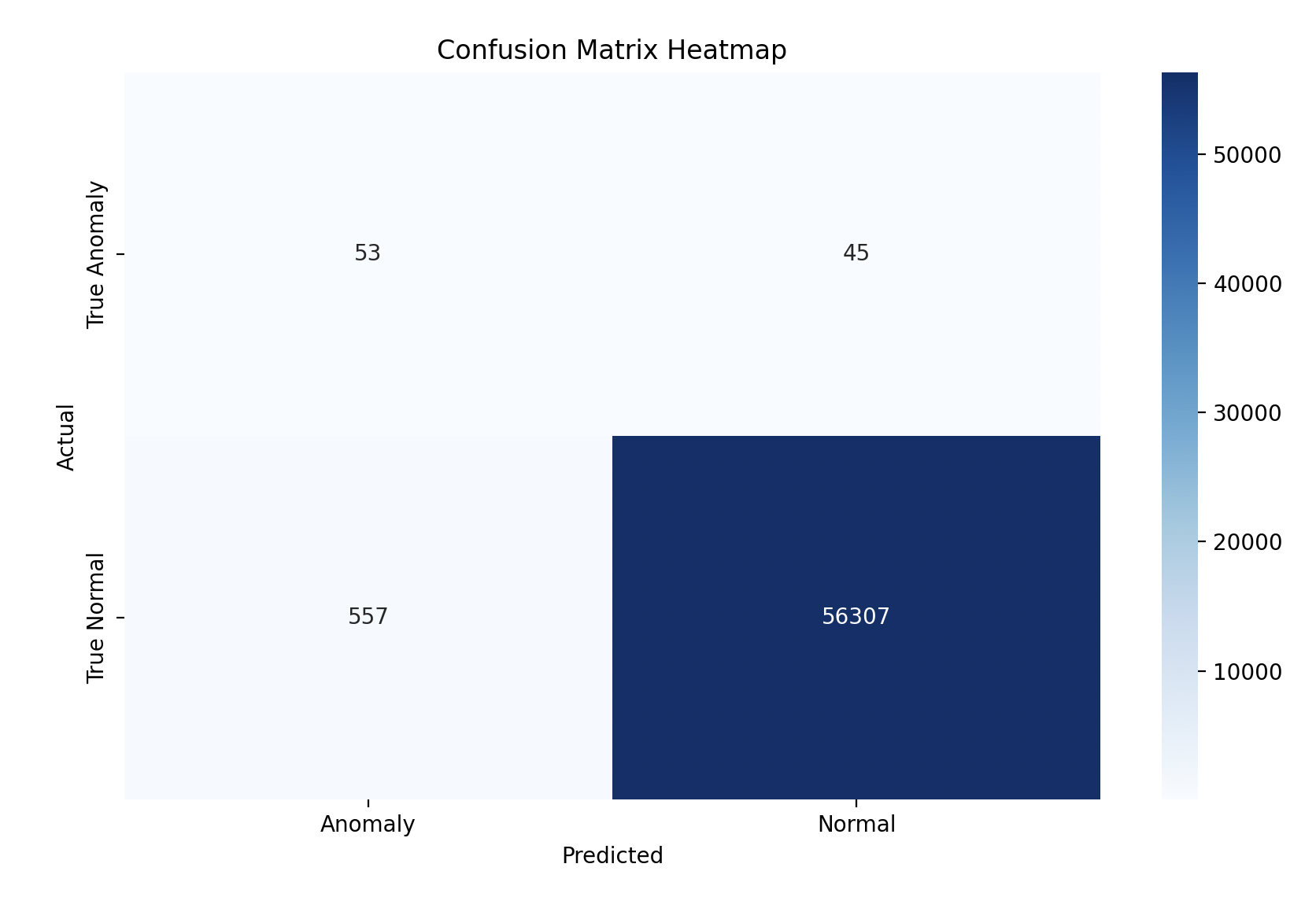
Confusion Matrix Heatmap:
plt.figure(figsize=(10, 6))
sns.heatmap(conf_matrix, annot=True, fmt='d', cmap='Blues', xticklabels=['Anomaly', 'Normal'], yticklabels=['True Anomaly', 'True Normal'])
plt.xlabel('Predicted')
plt.ylabel('Actual')
plt.title('Confusion Matrix Heatmap')
plt.show()
Model Performance
With 99% of accuracy the Isolation Forest model performed well in detecting anomalies. We can see a high rate of true normal transactions but some missed fraud cases and false positives.
Accuracy Score:
 0.989431550858467
Confusion Matrix:
 [[   53    45]
 [  557 56307]]
Classfication Report:
               precision    recall  f1-score   support

          -1       0.09      0.54      0.15        98
           1       1.00      0.99      0.99     56864

    accuracy                           0.99     56962
   macro avg       0.54      0.77      0.57     56962
weighted avg       1.00      0.99      0.99     56962
- 53 True Anomalies (Fraud) were correctly identified.
- 45 Fraud Cases were missed by the model.
- 557 False Positives were normal transactions mistakenly flagged as fraud.
- 56,307 True Normals were correctly identified as normal transactions.
Gratitude
Working with unsupervised learning and anomaly detection was a great learning experience. Stay tuned for Day 12!