Day 13 - 30 Days 30 ML Projects: Build a Music Genre Classifier Using Audio Features Extraction
The Problem
On Day 13 of the 30 Day 30 Machine Learning Projects Challenge, the goal was to build a model capable of classifying music into different genres based on audio features. The idea is to process audio files and extract specific characteristics from them, which can then be used to train a machine learning model that can predict genres.
If you want to see the code, you can find it here: GIT REPO.
Understanding the Data
We used the GTZAN Music Genre Dataset, which contains 1000 audio files (30 seconds each) across 10 genres: blues, classical, country, disco, hip-hop, jazz, metal, pop, reggae, and rock.
The audio files are stored in .wav format, and to train our model, we need to extract key audio features from the files like:
- MFCCs (Mel-frequency cepstral coefficients): Describes the short-term power spectrum of sound, which is crucial for identifying different genres.
- Spectral Contrast: Measures the difference between peaks and valleys in the sound spectrum.
- Chroma: Represents the pitch classes (e.g., C, C#, D, etc.) and is useful in recognizing harmonic and melodic elements.
Code Workflow
Here’s the step-by-step breakdown of the approach we followed:
- Load the Data and Extract Features
- Split the Data into Training and Validation Sets
- Build and Train the Model
- Make Predictions and Evaluate
- Visualize the Results
Before we start, import the required libraries:
import os
import librosa
import numpy as np
import pandas as pd
from sklearn.model_selection import train_test_split
from sklearn.ensemble import RandomForestClassifier
from sklearn.metrics import accuracy_score, confusion_matrix, classification_report
import matplotlib.pyplot as plt
import seaborn as sns
Step 1: Load the Data and Extract Features
We first downloaded the GTZAN Music Genre Dataset from the provided link. The audio files were categorized into subfolders based on their genre. We need only genes_original for this project. Unzip and place it in the dataset folder of your project. I have renamned it to genes. You can keep it if you desire but do change the name in the code:
Corrupted File Issue: During the process, we encountered an issue with the file /jazz/jazz.00054.wav, which was corrupted and had to be removed from the dataset before training.
dataset_path = 'dataset/genres/'
Feature extraction: To convert audio files into data that a machine learning model can understand, we extracted key features using the librosa library. Here’s a snippet showing how we extracted MFCCs and other features:
# Initialize lists to store features and labels.
features = []
labels = []

# Loop through each genre folder and load audio files.
for genre in os.listdir(dataset_path):
    genre_path = os.path.join(dataset_path, genre)
    for file in os.listdir(genre_path):
        file_path = os.path.join(genre_path, file)
        # Load the audio file and extract features
        y, sr = librosa.load(file_path, duration=30) # Load a 30 sec audio clip
        # Sample output:
        # y: [ 0.03451538  0.04815674  0.06430054 ... -0.03909302 -0.02001953 0.05392456]
        # sr: 22050

        # Extract features.
        mfcc = librosa.feature.mfcc(y = y, sr = sr, n_mfcc=13).mean(axis=1)
        chroma = librosa.feature.chroma_stft(y = y, sr = sr).mean(axis=1)
        contrast = librosa.feature.spectral_contrast(y = y, sr = sr).mean(axis=1)
        zcr = librosa.feature.zero_crossing_rate(y).mean()

        # Append to features labels list
        features.append(np.hstack([mfcc, chroma, contrast, zcr]))
        labels.append(genre)
Convert the features and labels lists into pandas Dataframe.
X = pd.DataFrame(features)
y = pd.Series(labels)
Step 2: Split the Data
We split the data into an 80% training set and a 20% test set, making sure that the training and validation datasets have a balanced distribution of genres.
X_train, X_val, y_train, y_val = train_test_split(X, y, test_size=0.2, random_state=42)
Step 3: Build and Train the Model
We trained a Random Forest Classifier with 100 decision trees. The Random Forest algorithm builds multiple decision trees and averages their predictions to make more accurate classifications.
model = RandomForestClassifier(n_estimators=100, random_state=42)
model.fit(X_train, y_train)
Step 4: Make Predictions and Evaluate
Once the model was trained, we predicted genres on the validation set and evaluated the results using accuracy, a confusion matrix, and a classification report.
predictions = model.predict(X_val)
accuracy_score = accuracy_score(y_val, predictions)
print("Accuracy Score:\n", accuracy_score)
confusion_matrix = confusion_matrix(y_val, predictions)
print("Confusion Matrix:\n", confusion_matrix)
classification_report = classification_report(y_val, predictions, zero_division=1)
print("Classification report:\n", classification_report)
Step 5: Visualization
plt.figure(figsize=(10, 7))
sns.heatmap(confusion_matrix, annot=True, fmt='d', cmap='Blues', xticklabels=y.unique(), yticklabels=y.unique())
plt.xlabel('Predicted Values')
plt.ylabel('Actual Values')
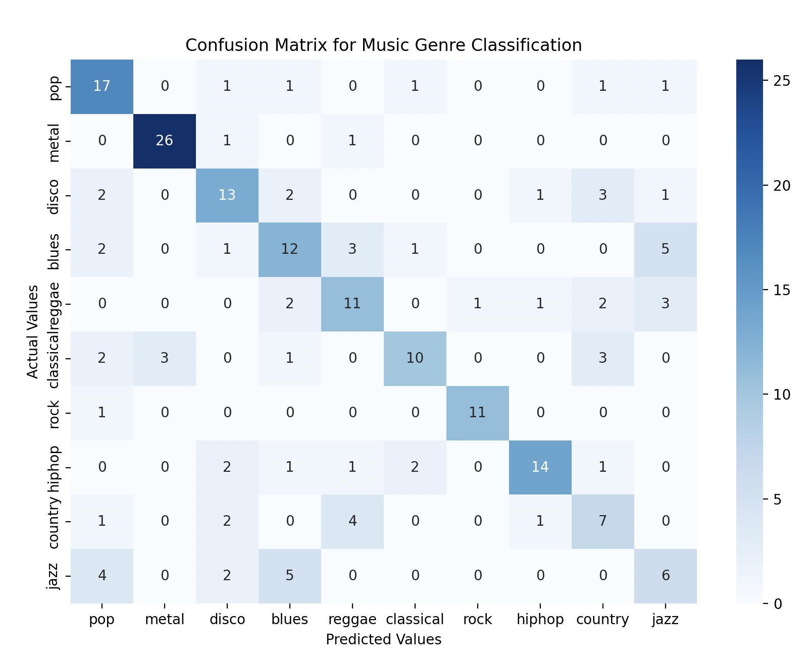
plt.title('Confusion Matrix for Music Genre Classification')
plt.show()
Model Performance
Accuracy Score:
 0.635
Confusion Matrix:
 [[17  0  1  1  0  1  0  0  1  1]
 [ 0 26  1  0  1  0  0  0  0  0]
 [ 2  0 13  2  0  0  0  1  3  1]
 [ 2  0  1 12  3  1  0  0  0  5]
 [ 0  0  0  2 11  0  1  1  2  3]
 [ 2  3  0  1  0 10  0  0  3  0]
 [ 1  0  0  0  0  0 11  0  0  0]
 [ 0  0  2  1  1  2  0 14  1  0]
 [ 1  0  2  0  4  0  0  1  7  0]
 [ 4  0  2  5  0  0  0  0  0  6]]
Classification report:
               precision    recall  f1-score   support

       blues       0.59      0.77      0.67        22
   classical       0.90      0.93      0.91        28
     country       0.59      0.59      0.59        22
       disco       0.50      0.50      0.50        24
      hiphop       0.55      0.55      0.55        20
        jazz       0.71      0.53      0.61        19
       metal       0.92      0.92      0.92        12
         pop       0.82      0.67      0.74        21
      reggae       0.41      0.47      0.44        15
        rock       0.38      0.35      0.36        17

    accuracy                           0.64       200
   macro avg       0.64      0.63      0.63       200
weighted avg       0.64      0.64      0.63       200
With Accuracy: 63.5%, you can see that the model performed best on classical and metal genres but struggled with rock and disco.
Gratitude
Today’s project helped me understand how audio features can be used to classify music genres. This was the second problem I solved using the RandomForestClassifier model, and remembering key points from the last problem made me feel like learning while coding is really working. I’m excited to solve more problems.
Stay Tuned!