Day 17 - 30 Days 30 ML Projects: Predict Diabetes Onset Using Decision Trees and Random Forests
On Day 17 of the 30 Days 30 Machine Learning Projects Challenge, the task was to predict whether a person would develop diabetes based on various medical factors such as glucose levels, insulin levels, and age. This is a binary classification problem where the goal is to predict if a person is diabetic (1) or not (0).
If you want to see the code, you can find it here: GIT REPO.
Understanding the Data
We used the Pima Indians Diabetes Dataset, which includes medical records of women aged 21 and above. The dataset contains various features related to pregnancies, glucose levels, blood pressure, skin thickness, and more. Here’s a glimpse of the data:
   Pregnancies  Glucose  BloodPressure  SkinThickness  Insulin   BMI  DiabetesPedigreeFunction  Age  Outcome
0            6      148             72             35        0  33.6                     0.627   50        1
1            1       85             66             29        0  26.6                     0.351   31        0
2            8      183             64              0        0  23.3                     0.672   32        1
3            1       89             66             23       94  28.1                     0.167   21        0
4            0      137             40             35      168  43.1                     2.288   33        1
Outcome:
- 1 means the patient is diabetic.
- 0 means the patient is not diabetic.
Code Workflow
Here’s the step-by-step breakdown of how I approached this problem:
Step 1: Load the Data
First, I loaded the dataset using Pandas to explore and understand the data.
import pandas as pd

# Load the dataset
data = pd.read_csv('dataset/diabetes.csv')
print(data.head())
Step 2: Preprocess the Data
Next, I separated the features (X) from the target (y).
X = data.drop('Outcome', axis=1)  # Features
y = data['Outcome']  # Target
Step 3: Split the Data
The data was then split into training and validation sets with an 80-20 split.
from sklearn.model_selection import train_test_split

X_train, X_val, y_train, y_val = train_test_split(X, y, test_size=0.2, random_state=42)
Step 4: Build and Train the Models
Decision Tree: I trained a Decision Tree Classifier as the first model.
from sklearn.tree import DecisionTreeClassifier

# Build and train the Decision Tree model
decision_tree = DecisionTreeClassifier(random_state=42)
decision_tree.fit(X_train, y_train)
Random Forest: Next, I trained a Random Forest Classifier with 100 trees and specific parameters.
from sklearn.ensemble import RandomForestClassifier

# Build and train the Random Forest model
random_forest = RandomForestClassifier(n_estimators=100, min_samples_leaf=1, min_samples_split=5, random_state=42)
random_forest.fit(X_train, y_train)
Step 5: Make Predictions and Evaluate
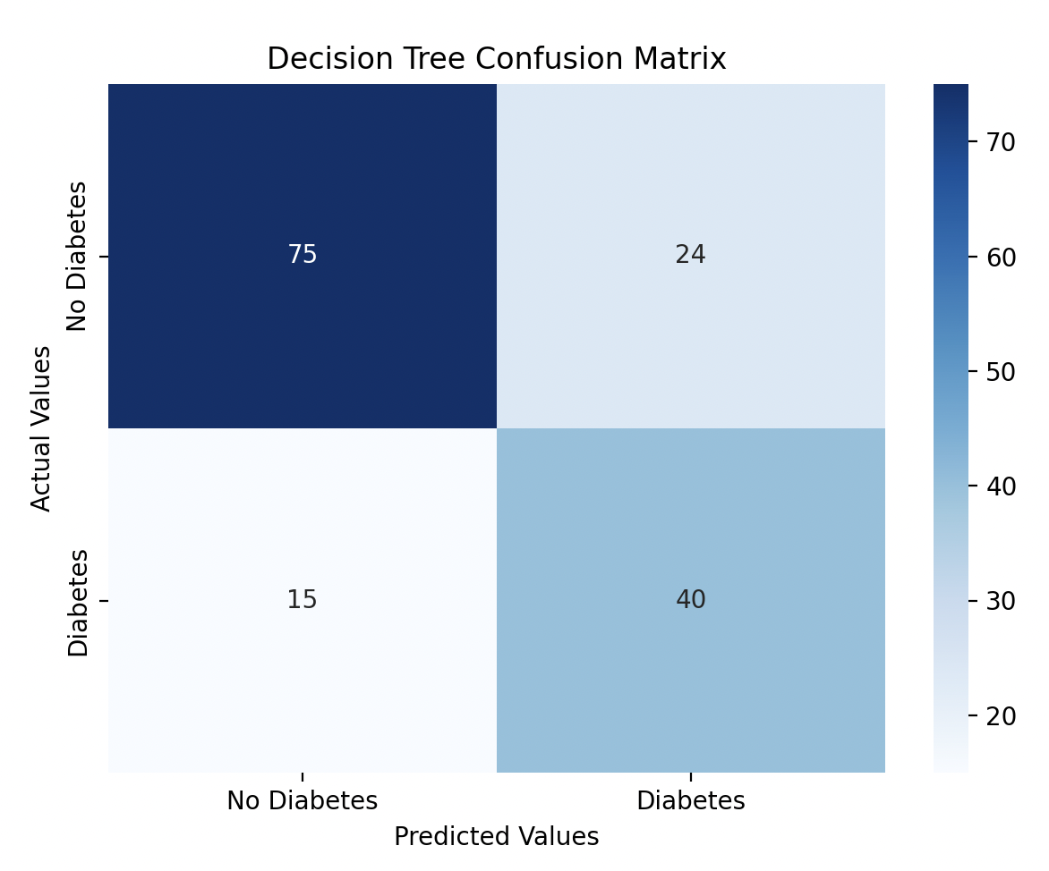
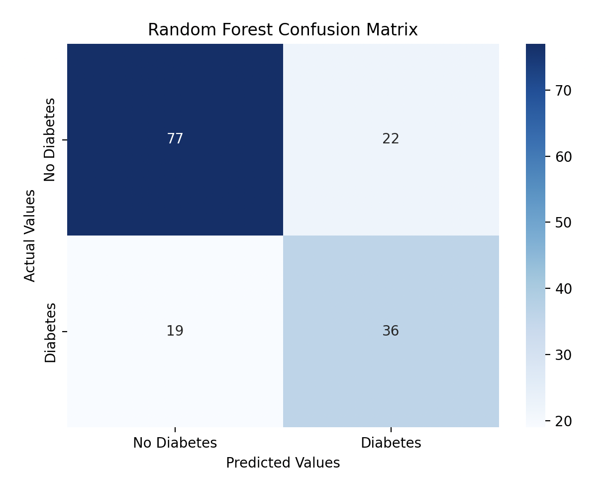
After training, I made predictions on the validation set and evaluated both models using accuracy, confusion matrices, and classification reports.
from sklearn.metrics import accuracy_score, confusion_matrix, classification_report

# Decision Tree
dt_predictions = decision_tree.predict(X_val)
dt_accuracy = accuracy_score(y_val, dt_predictions)
dt_confusion_matrix = confusion_matrix(y_val, dt_predictions)
dt_classification_report = classification_report(y_val, dt_predictions)

print(f"Decision Tree Accuracy Score: {dt_accuracy}")
print(f"Decision Tree Confusion Matrix: {dt_confusion_matrix}")
print(f"Decision Tree Classification Report: {dt_classification_report}")

# Random Forest
rf_predictions = random_forest.predict(X_val)
rf_accuracy = accuracy_score(y_val, rf_predictions)
rf_confusion_matrix = confusion_matrix(y_val, rf_predictions)
rf_classification_report = classification_report(y_val, rf_predictions)

print(f"Random Forest Accuracy Score: {rf_accuracy}")
print(f"Random Forest Confusion Matrix: {rf_confusion_matrix}")
print(f"Random Forest Classification Report: {rf_classification_report}")
Results:
- Decision Tree Accuracy: 74%
- Random Forest Accuracy: 73%
Step 6: Visualization
I visualized the confusion matrices for both models using Seaborn heatmaps.
import matplotlib.pyplot as plt
import seaborn as sns

# Decision Tree
plt.figure(figsize=(7, 5))
sns.heatmap(dt_confusion_matrix, annot=True, fmt='d', cmap='Blues', xticklabels=['No Diabetes', 'Diabetes'], yticklabels=['No Diabetes', 'Diabetes'])
plt.xlabel('Predicted Values')
plt.ylabel('Actual Values')
plt.title('Decision Tree Confusion Matrix')
plt.show()

# Random Forest
plt.figure(figsize=(7, 5))
sns.heatmap(rf_confusion_matrix, annot=True, fmt='d', cmap='Blues', xticklabels=['No Diabetes', 'Diabetes'], yticklabels=['No Diabetes', 'Diabetes'])
plt.xlabel('Predicted Values')
plt.ylabel('Actual Values')
plt.title('Random Forest Confusion Matrix')
plt.show()


Model Performance
The Decision Tree performed slightly better with a 74% accuracy score, while the Random Forest model performed at 73% accuracy. I tried improving the Random Forest model by performing hyperparameter tuning.
from sklearn.model_selection import GridSearchCV

param_grid = {
    'n_estimators': [100, 200],
    'max_depth': [None, 10, 20],
    'min_samples_split': [2, 5],
    'min_samples_leaf': [1, 2]
}

grid_search = GridSearchCV(estimator=rf, param_grid=param_grid, cv=5, n_jobs=-1, verbose=2)
grid_search.fit(X_train, y_train)

# Display the best parameters and score
print("Best Parameters:", grid_search.best_params_)
print("Best Score:", grid_search.best_score_)
After tuning, the best parameters were:
Best Parameters: {'max_depth': None, 'min_samples_leaf': 1, 'min_samples_split': 5, 'n_estimators': 100}
Best Score: 0.783
However, the model’s accuracy remained consistent at 73%.
Gratitude
This project was a deep dive into comparing Decision Trees and Random Forests. I learned a lot about tuning models and how important it is to understand the trade-offs between complexity and performance.
Stay tuned for Day 18!