Day 18 - 30 Days 30 ML Projects: Time Series Forecasting of Stock Prices With ARIMA Model
On Day 18 of the 30 Days 30 Machine Learning Projects Challenge, the task was to predict stock prices using the ARIMA model. ARIMA (Auto-Regressive Integrated Moving Average) is one of the most widely used techniques for time series forecasting, especially for data that shows trends or seasonality.
If you want to see the code, you can find it here: GIT REPO.
Understanding the Data
We used the MAANG Historical Stock Market Dataset and worked specifically with Apple stock prices. The dataset contains various columns, but for this project, we used the Close price, which represents the final trading price of the stock on each day.
Code Workflow
Below is the step-by-step approach followed for solving this problem.
Step 1: Load the Data and Preprocess
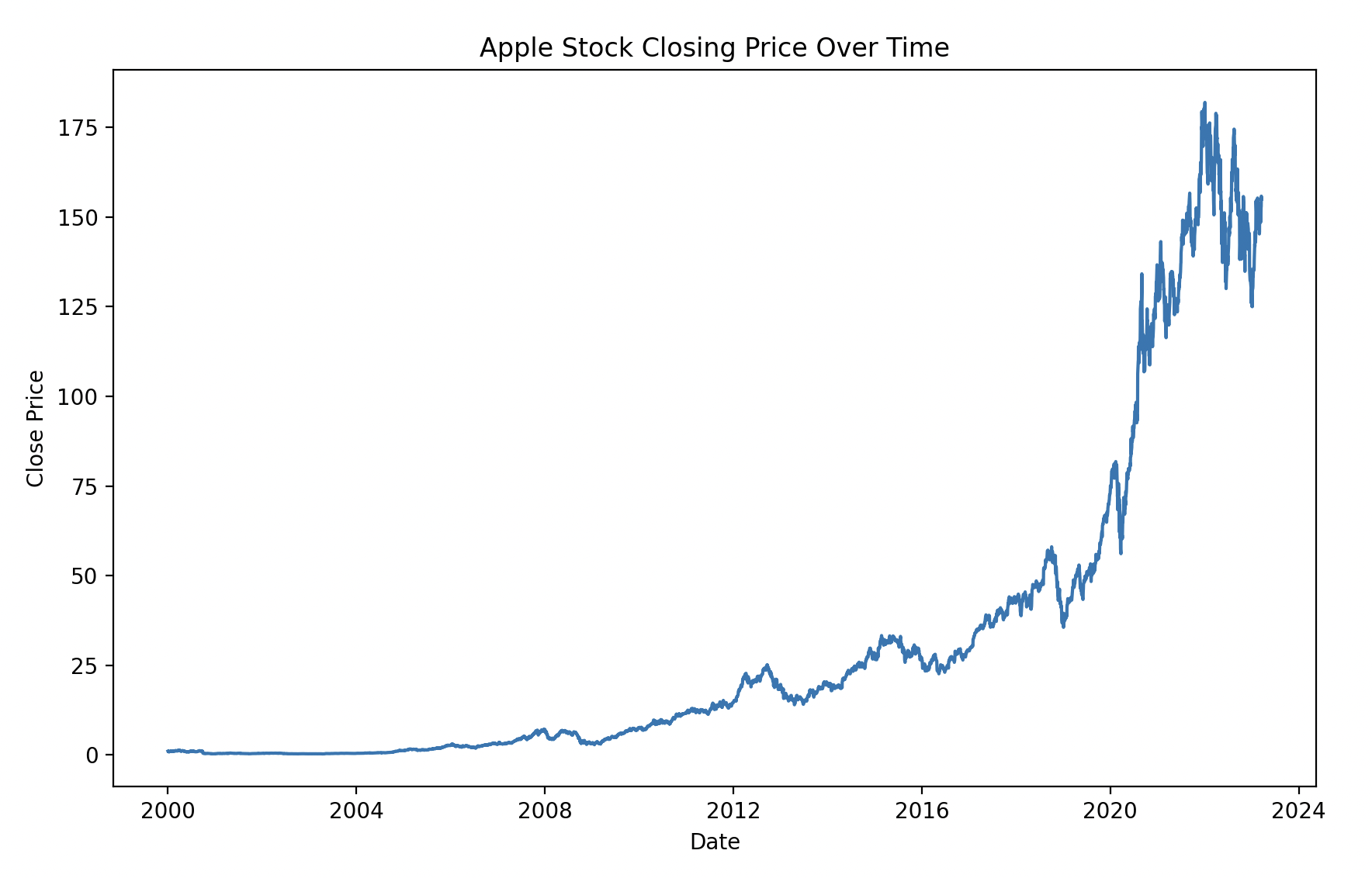
We’ll load the Apple stock dataset and focus on the ‘Date’ and ‘Close’ columns to predict future stock prices. Since ARIMA requires a continuous time series, we’ll set the ‘Date’ column as the index.
import pandas as pd
import matplotlib.pyplot as plt
from statsmodels.tsa.arima.model import ARIMA
from pandas.plotting import autocorrelation_plot
import warnings

warnings.filterwarnings("ignore")

# Load the data
data = pd.read_csv('dataset/Apple.csv')

# Convert the 'Date' column to datetime format and set it as the index
data['Date'] = pd.to_datetime(data['Date'])
data.set_index('Date', inplace=True)

# Plot the closing price to visualize the time series
plt.figure(figsize=(10,6))
plt.plot(data['Close'], label='Apple Stock Closing Price')
plt.title('Apple Stock Closing Price Over Time')
plt.xlabel('Date')
plt.ylabel('Close Price')
plt.legend()
plt.show()
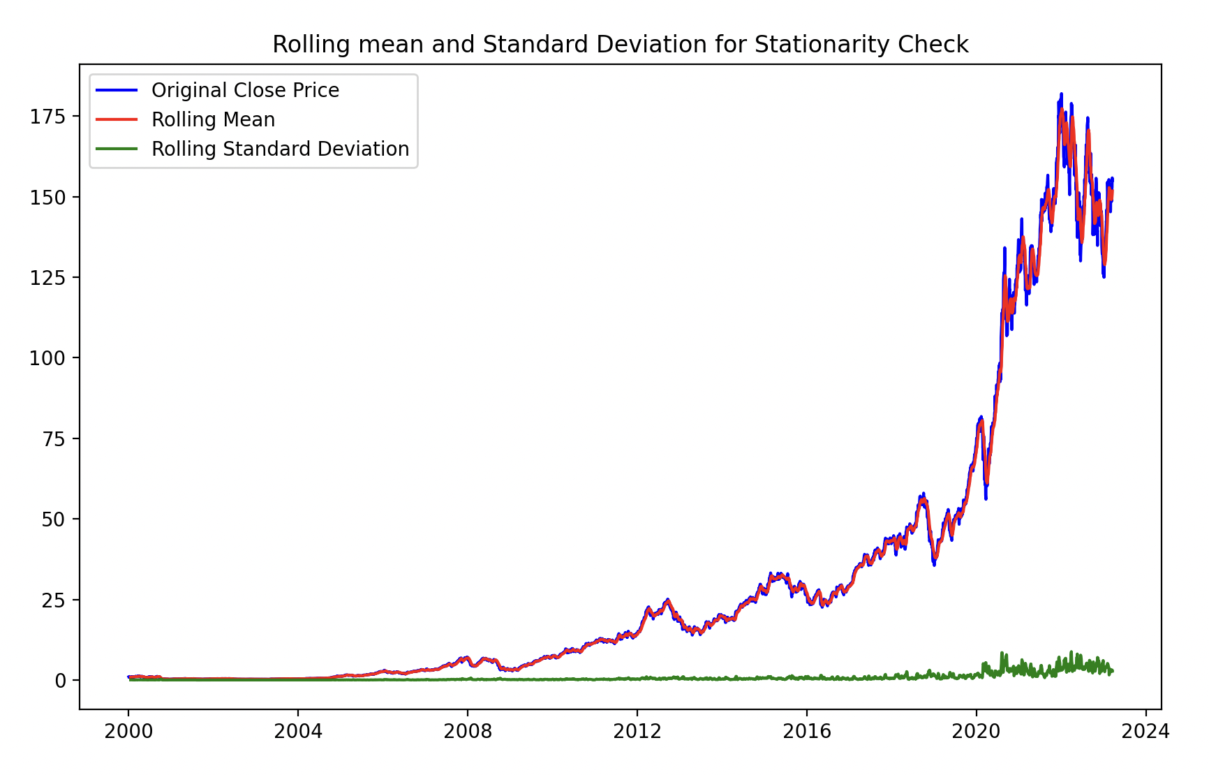
Step 2: Check for Stationarity
For ARIMA to work well, we need a stationary time series. We’ll check for stationarity using a rolling mean and standard deviation.
# Calculate rolling statistics to check for stationarity
rolling_mean = data['Close'].rolling(window=12).mean()
rolling_std = data['Close'].rolling(window=12).std()

# Plot rolling statistics
plt.figure(figsize=(10,6))
plt.plot(data['Close'], color='blue', label='Original Close Price')
plt.plot(rolling_mean, color='red', label='Rolling Mean')
plt.plot(rolling_std, color='black', label='Rolling Std')
plt.title('Rolling Mean & Standard Deviation for Stationarity Check')
plt.legend()
plt.show()
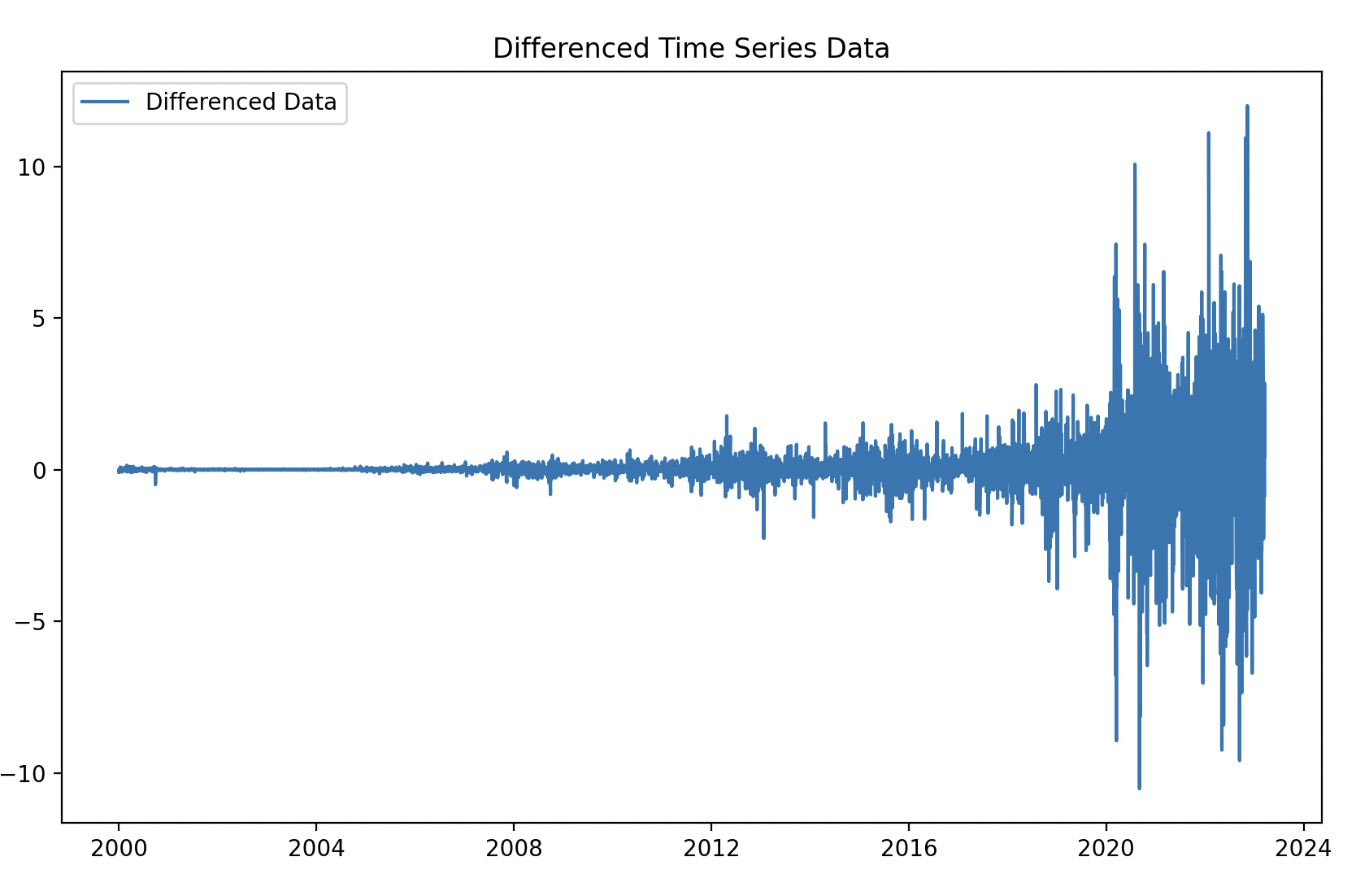
Step 3: Differencing the Data to Make it Stationary
If the data is not stationary, we’ll apply differencing to remove trends and seasonality.
# Differencing the data to make it stationary
data_diff = data['Close'].diff().dropna()

# Plot the differenced data
plt.figure(figsize=(10,6))
plt.plot(data_diff, label='Differenced Data')
plt.title('Differenced Time Series Data')
plt.legend()
plt.show()
Step 4: Fit the ARIMA Model
Now that we have stationary data, we can fit an ARIMA model to it. We’ll use ARIMA’s parameters (p, d, q) to control the autoregression (AR), differencing (I), and moving average (MA) parts.
# Fit the ARIMA model
model = ARIMA(data['Close'], order=(5, 1, 0))  # You can experiment with other (p, d, q) values
model_fit = model.fit()

# Summary of the model
print(model_fit.summary())
let’s decode the parameters (p=5, d=1, q=0):
p (Auto-Regressive part): Looks at the number of lag observations included in the model. d (Differencing part): Indicates how many times the data needs to be differenced to make it stationary. q (Moving Average part): Determines the size of the moving average window.
Step 5: Make Predictions
We forecasted the next 30 days of Apple stock prices and plotted the predictions against the actual prices.
# Forecast future prices
forecast = model_fit.forecast(steps=30)  # Forecast for 30 days ahead
plt.figure(figsize=(10,6))
plt.plot(data['Close'], label='Actual Prices')
plt.plot(forecast, label='Predicted Prices', color='red')
plt.title('Apple Stock Price Prediction with ARIMA')
plt.xlabel('Date')
plt.ylabel('Close Price')
plt.legend()
plt.show()
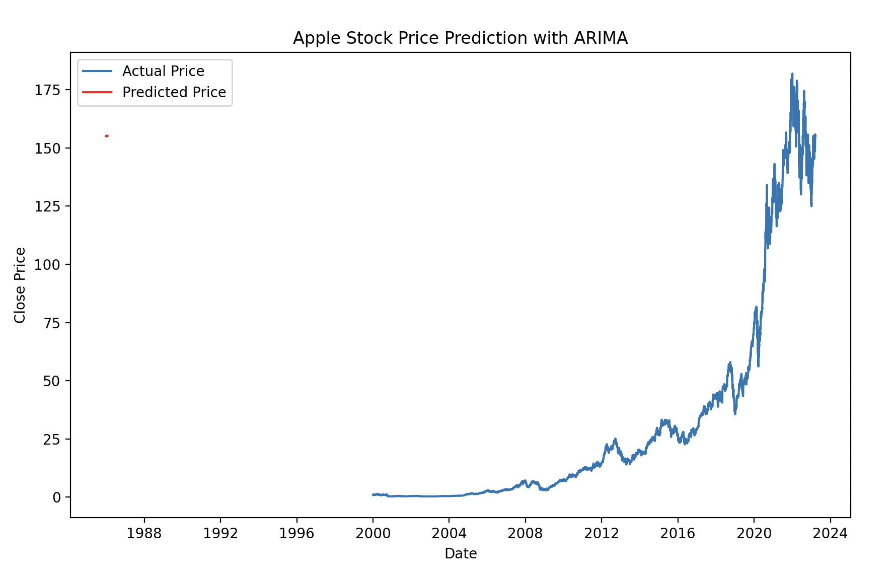
The ARIMA model was able to predict short-term future values for Apple stock prices.
Gratitude
It was really exciting working with ARIMA to predict stock prices! Looking forward to tomorrow’s challenge!
Stay Tuned!