Day 25 - Sentiment Analysis of Customer Reviews Using Traditional NLP Techniques
For today’s task, I performed Sentiment Analysis on customer reviews using traditional Natural Language Processing (NLP) techniques. The goal was to classify customer reviews from the IMDb Movie Reviews Dataset as either positive or negative using preprocessing, feature extraction with TF-IDF, and a simple Logistic Regression model.
If you want to see the code, you can find it here: GIT REPO.
Dataset:
I used the IMDb Dataset of 50K Movie Reviews, which contains 50,000 reviews, each labeled as either positive or negative.
Steps Taken:
Let’s import the libraries first.
import pandas as pd
import re
from nltk.tokenize import word_tokenize
from nltk.corpus import stopwords
from nltk.stem import PorterStemmer
from sklearn.model_selection import train_test_split
from sklearn.feature_extraction.text import TfidfVectorizer
from sklearn.linear_model import LogisticRegression
from sklearn.metrics import accuracy_score, confusion_matrix, classification_report
import matplotlib.pyplot as plt
import seaborn as sns
Step 1: Load the Data
I started by loading the dataset and inspecting the first few rows. The dataset contains two columns: review (text data) and sentiment (positive/negative labels).
data = pd.read_csv('dataset/IMDB_Dataset.csv')
Step 2: Data Preprocessing
Next, I preprocessed the text data to clean and normalize it for analysis. The preprocessing steps included:
- Removing HTML tags and special characters.
- Lowercasing the text.
- Tokenizing the text into words.
- Removing stopwords (common words that don’t contribute much to meaning, e.g., “the”, “and”).
- Stemming the words using PorterStemmer, which reduces words to their root form (e.g., “running” to “run”).
This was done to reduce noise in the text and focus on the core words contributing to sentiment.
def preprocesss_text(text):
    # Remove the HTMl tags and special characters.
    text = re.sub(r'<.*?>', '', text)  # <html> <body> etc
    text = re.sub(r'[^\w\s]', '', text)

    # Convert to lower.
    text = text.lower()

    # Tokenize
    tokens = word_tokenize(text)

    # Remove the stopwords and apply stemming.
    stop_words = set(stopwords.words('english'))
    tokens = [word for word in tokens if word not in stop_words] # Remove stopwords
    stemmer = PorterStemmer()
    tokens = [stemmer.stem(word) for word in tokens] # Applied stemming.

    return ' '.join(tokens)

# Apply preprocessing on the reviews feature
data['cleaned_review'] = data['review'].apply(preprocesss_text)
Step 3: Create Features and Target Datasets
After preprocessing the text, I created two main components:
- Features (X): The cleaned reviews (text after preprocessing).
- Target (y): The sentiment (positive/negative) corresponding to each review.
These will be used to train and evaluate the model.
X = data['cleaned_review']  # Feature: Cleaned reviews
y = data['sentiment']       # Target: Sentiment (positive/negative)
Step 4: Split the Data into Training and Validation Sets
I split the data into training (80%) and validation (20%) sets to evaluate the model’s performance. This ensures that the model is trained on one part of the data and tested on unseen data to measure generalization.
X_train, X_val, y_train, y_val = train_test_split(X, y, test_size=0.2, random_state=42)
Step 5: Feature Extraction Using TF-IDF
To convert the text into numerical form, I used TF-IDF (Term Frequency-Inverse Document Frequency), which captures the importance of words in the corpus. I applied the TF-IDF vectorizer on the training data and transformed both the training and validation sets.
tfidf_vectorizer = TfidfVectorizer(max_features=5000)
X_train_tfidf = tfidf_vectorizer.fit_transform(X_train)
X_val_tfidf = tfidf_vectorizer.transform(X_val)
Step 6: Train the Model
I used Logistic Regression to build the sentiment analysis model. Logistic Regression is a popular choice for text classification tasks due to its simplicity and effectiveness.
model = LogisticRegression()
model.fit(X_train_tfidf, y_train)
Step 7: Make Prediction Evaluate the Model
After training the model, I made predictions on the validation set and evaluated its performance using accuracy, a confusion matrix, and a classification report (precision, recall, F1-score).
predictions = model.predict(X_val_tfidf)

accuracy_score = accuracy_score(y_val, predictions)
confusion_matrix = confusion_matrix(y_val, predictions)
classification_report = classification_report(y_val, predictions)

print(f"Accuracy Score: \n {accuracy_score}")
print(f"Confusion Matrix: \n {confusion_matrix}")
print(f"Classification Report: \n {classification_report}")
Output
# Output
# Accuracy Score:
#  0.8848
# Confusion Matrix:
#  [[4304  657]
#  [ 495 4544]]
# Classification Report:
#                precision    recall  f1-score   support
#
#     negative       0.90      0.87      0.88      4961
#     positive       0.87      0.90      0.89      5039
#
#     accuracy                           0.88     10000
#    macro avg       0.89      0.88      0.88     10000
# weighted avg       0.89      0.88      0.88     10000
Accuracy: The model achieved an accuracy of 88.48% on the validation set.
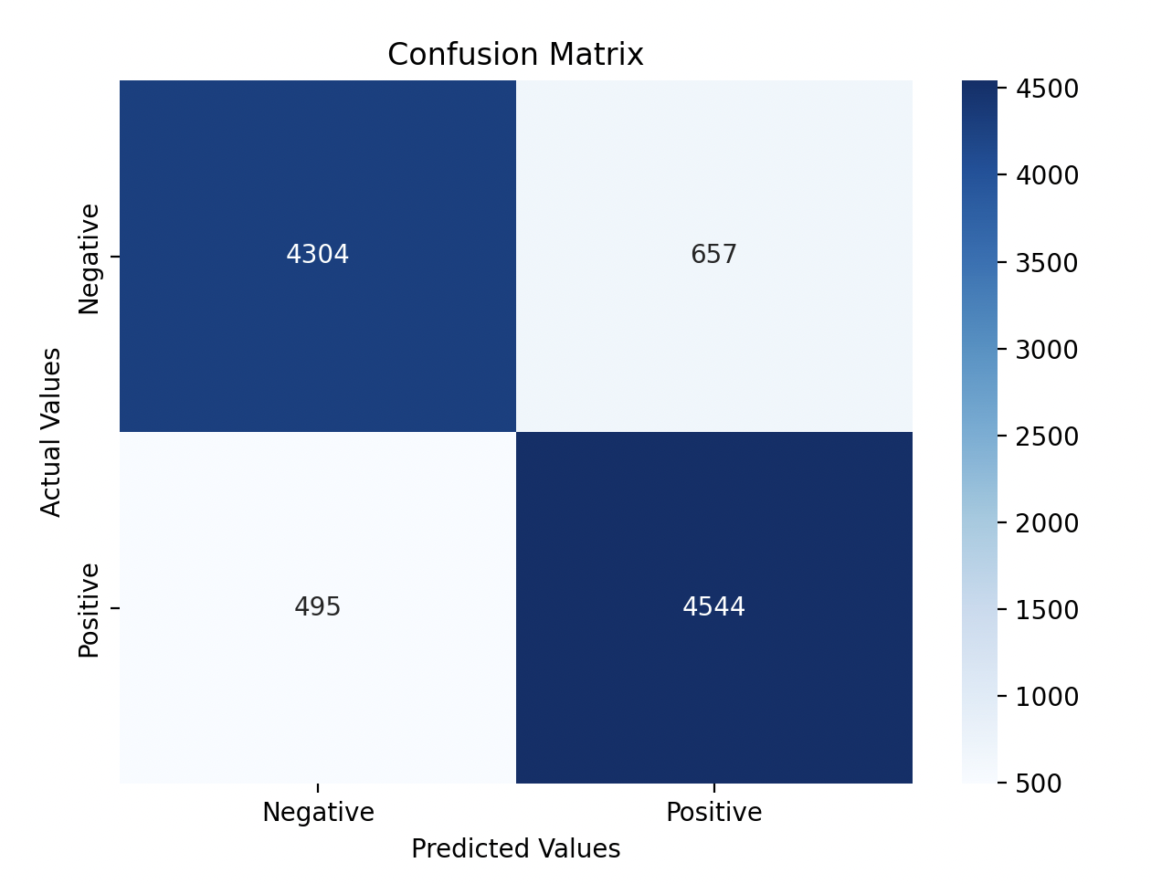
Confusion Matrix: Showed that the model correctly classified most reviews, with some false positives and false negatives.
- The model correctly classified 4304 negative reviews and 4544 positive reviews.
- There were 657 false positives (where the model incorrectly classified negative reviews as positive) and 495 false negatives (where the model incorrectly classified positive reviews as negative).
Classification Report: Provided detailed metrics like precision, recall, and F1-score for both positive and negative sentiments.
- Negative Precision = 0.90: Out of all reviews predicted as negative, 90% were actually negative.
- Positive Precision = 0.87: Out of all reviews predicted as positive, 87% were actually positive.
- Negative Recall = 0.87: Out of all actual negative reviews, 87% were correctly predicted as negative.
- Positive Recall = 0.90: Out of all actual positive reviews, 90% were correctly predicted as positive.
- Negative F1-Score = 0.88: The F1-score for negative reviews shows a balance between precision (0.90) and recall (0.87).
- Positive F1-Score = 0.89: The F1-score for positive reviews also shows a good balance between precision (0.87) and recall (0.90).
- Negative Support = 4961: There were 4961 actual negative reviews in the validation set.
- Positive Support = 5039: There were 5039 actual positive reviews in the validation set.
Step 8: Visualization
I visualized the confusion matrix to get a clearer understanding of how the model performed. The confusion matrix shows how many reviews were correctly classified as positive or negative, and where the model made errors.
plt.figure(figsize=(7, 5))
sns.heatmap(confusion_matrix, annot=True, fmt='d', cmap='Blues', xticklabels=['Negative','Positive'], yticklabels=['Negative','Positive'])
plt.xlabel('Predicted Values')
plt.ylabel('Actual Values')
plt.title('Confusion Matrix')
plt.show()
Gratitude
Although we have performed all the above steps in many of our previous problems, this being the first problem in NLP, it was great to learn what is needed to get started. I’m looking forward to the next problem.
Stay Tuned!