Day 26- Time Series Forecasting of Electricity Consumption Using LSTM (Intro to Deep Learning)
Today’s task was to use LSTM (Long Short-Term Memory), a type of Recurrent Neural Network (RNN), to forecast electricity consumption based on historical data. This project served as an introduction to deep learning for time series forecasting, where LSTMs excel at capturing long-term dependencies in sequential data.
If you want to see the code, you can find it here: GIT REPO.
Dataset:
I used the AEP Hourly Dataset from Kaggle’s Hourly Energy Consumption Dataset problem, which consists of 121,273 hourly electricity consumption records in megawatts (MW). The goal was to predict future electricity consumption based on past hourly data.
Code Flow:
- Load and inspect the dataset.
- Convert the Datetime column to the correct format.
- Handle missing values (if any).
- Normalize the AEP_MW column for better model performance.
- Create sequences for the LSTM model (sliding windows).
- Split the data into training and test sets.
- Train the LSTM model and make predictions.
- Visualize the results.
Step 1: Load and Convert Datetime
We’ll start by loading the dataset and converting the Datetime column to a datetime object so that we can handle it easily in the future if we need to. This will allow us to index by time if needed.
import pandas as pd

# Load the data
data = pd.read_csv('dataset/AEP_hourly.csv')

# Convert 'Datetime' column to datetime object
data['Datetime'] = pd.to_datetime(data['Datetime'])

# Set the 'Datetime' column as the index
data.set_index('Datetime', inplace=True)

# Check for any missing values
print(data.isnull().sum())
Step 2: Handle Missing Values (if any)
Check if there are any missing values. If there are, we can either drop them or use interpolation to fill them.
# Handle missing values by interpolating
data = data.interpolate()

# Drop any remaining missing values
data = data.dropna()
If there are no missing values, you can skip this step.
Step 3: Normalize the Data
It’s crucial to normalize the AEP_MW values to a range between 0 and 1. This helps the LSTM model converge faster and perform better.
from sklearn.preprocessing import MinMaxScaler

# Select the 'AEP_MW' column for normalization
scaler = MinMaxScaler(feature_range=(0, 1))
scaled_data = scaler.fit_transform(data[['AEP_MW']])

# Check the first few rows of the scaled data
print(scaled_data[:5])
Step 4: Create Sequences for the LSTM Model
We’ll use sliding windows of, for example, 60 hours to predict the next hour of electricity consumption. The create_sequences function will help us transform the data into the format needed for LSTM.
import numpy as np

# data: The entire time series data (in this case, the scaled electricity consumption data).
# time_steps: The number of previous time steps (hours) you want to use as input to predict the next time step.
def create_sequences(data, time_steps):
    sequences = [] # This list will store the input sequences (i.e., the previous 60 hours of electricity consumption).
    target = [] # This list will store the corresponding target values.

    for i in range(len(data) - time_steps):
        sequences.append(data[i: i + time_steps])
        target.append(data[i + time_steps])

    return np.array(sequences), np.array(target)

# Set time_steps to 60 (using the previous 60 hours to predict the next hour)
time_steps = 60

# Create sequences
X, y = create_sequences(scaled_data, time_steps)

# Check the shape of the sequences
print(X.shape, y.shape)
Step 5: Split the Data into Training and Test Sets
We’ll split the data into 80% training and 20% test sets to ensure the model is trained on historical data and tested on future data.
# Split the data into training and test sets (80% train, 20% test)
train_size = int(len(X) * 0.8)
X_train, X_test = X[:train_size], X[train_size:]
y_train, y_test = y[:train_size], y[train_size:]

# Check the shape of the train/test sets
print(X_train.shape, X_test.shape)
Step 6: Build and Train the LSTM Model
Now, we can build a simple LSTM model using Keras. We’ll use 50 units in the LSTM layer, followed by a dense layer to output the predicted value.
import tensorflow as tf
from tensorflow.keras.models import Sequential
from tensorflow.keras.layers import LSTM, Dense

# Create the LSTM model
model = Sequential()

# Add an LSTM layer with 50 units
model.add(LSTM(50, return_sequences=False, input_shape=(X_train.shape[1], 1)))

# Add a Dense layer to output a single value (the predicted consumption)
model.add(Dense(1))

# Compile the model
model.compile(optimizer='adam', loss='mean_squared_error')

# Train the model
history = model.fit(X_train, y_train, epochs=20, batch_size=32, validation_data=(X_test, y_test))
Step 7: Evaluate the Model
Once the model is trained, we can evaluate it by making predictions on the test set.
# Make prediction
predictions = model.predict(X_val)

# Transforms the predicted values from the scaled range (0-1) back to the original range, which represents real
# electricity consumption values in MW.
predictions = scaler.inverse_transform(predictions)
y_val_org = scaler.inverse_transform(y_val.reshape(-1, 1))

# Visualization
plt.figure(figsize=(10, 7))
plt.plot(y_val_org, label="Actual Consumption")
plt.plot(predictions, label="Predicted Consumption")
plt.xlabel('Time')
plt.ylabel('Consumption (MW)')
plt.title('Electricity Consumption Forecasting')
plt.legend()
plt.show()
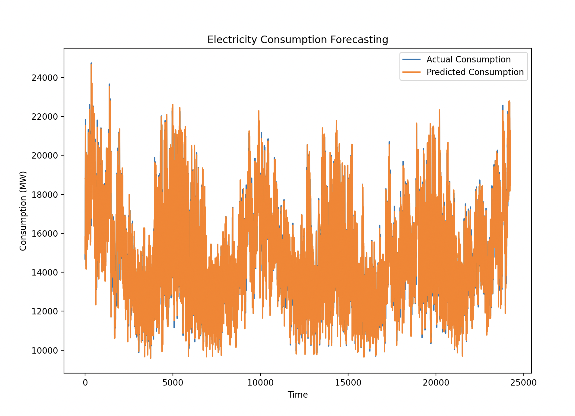
The plot showed the actual and predicted electricity consumption values overlapping closely, indicating that the LSTM model captured the underlying patterns quite well. Both short-term and long-term trends were effectively modeled, with only minor deviations.
Results:
The model was able to closely track the actual electricity consumption, with minor prediction errors, as seen in the plot where the orange line (predicted consumption) closely followed the blue line (actual consumption). The overall performance suggests that the LSTM model is well-suited for this type of time series forecasting problem.
Gratitude
Being the first problem in deep learning, it was exciting to understand and explore new topics. I plan to start a dedicated challenge on deep learning after this one finishes. I also can’t wait to tackle all the problems in this challenge.
Stay Tuned!