Day 27 - Image Classification With a Small CNN on CIFAR-10 Dataset

The task for Day 27 was to build a Convolutional Neural Network (CNN) for image classification on the CIFAR-10 dataset. The CIFAR-10 dataset consists of 60,000 32x32 color images in 10 different classes, such as airplanes, cars, birds, and cats. The goal was to create a small CNN to classify these images into the correct categories and evaluate its performance.

If you want to see the code, you can find it here: GIT REPO.

Dataset:

The CIFAR-10 dataset contains:

50,000 training images and 10,000 test images.
Images are 32x32 pixels with 3 color channels (RGB).
Each image belongs to one of 10 classes.

Steps Taken:

Step 1: Load and Preprocess the Data

I loaded the CIFAR-10 dataset using TensorFlow’s built-in dataset utility. The images were normalized by scaling the pixel values from 0-255 to a range of [0, 1] to ensure that the model learns efficiently. The labels were one-hot encoded, which converted the categorical labels into binary vectors for use in multi-class classification.

(X_train, y_train), (X_val, y_val) = cifar10.load_data()

X_train = X_train.astype('float32') / 255.0
X_val = X_val.astype('float32') / 255.0

y_train = to_categorical(y_train, 10)
y_val = to_categorical(y_val, 10)

Step 2: Build a Small CNN Architecture

I created a Sequential model with 3 convolutional layers followed by MaxPooling layers to reduce spatial dimensions. Each convolutional layer used ReLU activation, and the number of filters increased with each layer to capture more complex features.

I used a Dense (fully connected) layer with 128 units and Dropout to prevent overfitting. Finally, the model used a softmax output layer to output probabilities for each of the 10 classes.

model = Sequential()
model.add(Conv2D(32, (3, 3), activation='relu', input_shape=(32, 32, 3)))
model.add(MaxPooling2D(2, 2))

model.add(Conv2D(64, (3, 3), activation='relu'))
model.add(MaxPooling2D(2, 2))

model.add(Conv2D(128, (3, 3), activation='relu'))
model.add(MaxPooling2D(2, 2))

model.add(Flatten())
model.add(Dense(128, activation='relu'))
model.add(Dropout(0.5))
model.add(Dense(10, activation='softmax'))

Step 3: Compile the Model

I compiled the model using Adam optimizer and categorical crossentropy as the loss function (because it’s a multi-class classification problem). The model was also configured to track accuracy as a performance metric.

model.compile(optimizer='adam', loss='categorical_crossentropy', metrics=['accuracy'])

Step 4: Train the Model

The model was trained for 10 epochs with a batch size of 64 using 80% of the data for training and 20% for validation. During training, both the accuracy and loss were tracked for both the training and validation sets.

history = model.fit(X_train, y_train, epochs=10, batch_size=64, validation_data=(X_val, y_val))

Step 5: Evaluate the Model and Visualize the Results

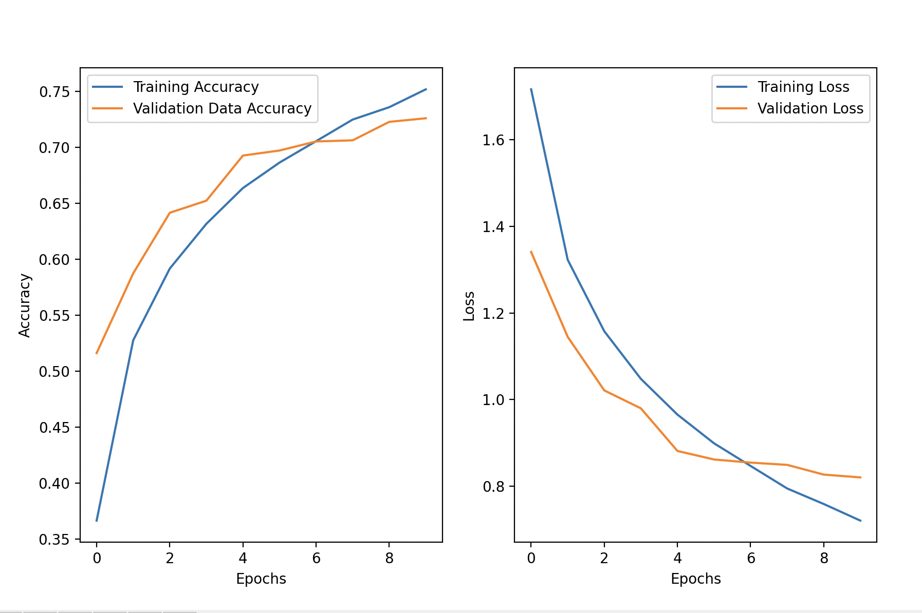
After training, I evaluated the model on the test set. The validation accuracy reached 72.58%, indicating that the model performed reasonably well for a basic CNN architecture on CIFAR-10.

Model Architecture and Performance:

Epoch 1/10: val_accuracy: 0.5161
Epoch 5/10: val_accuracy: 0.6925
Epoch 10/10: val_accuracy: 0.7258
Validation Accuracy: 0.7258

The training and validation curves show consistent improvement, with no significant overfitting observed. Here are the accuracy and loss plots over the epochs:

val_loss, val_acc = model.evaluate(X_val, y_val)
print(f"Validation Accuracy: {val_acc}")

plt.figure(figsize=(10, 6))

# Plot accuracy
plt.subplot(1, 2, 1)
plt.plot(history.history['accuracy'], label="Training Accuracy")
plt.plot(history.history['val_accuracy'], label="Validation Accuracy")
plt.xlabel('Epochs')
plt.ylabel('Accuracy')
plt.legend()

# Plot loss
plt.subplot(1, 2, 2)
plt.plot(history.history['loss'], label="Training Loss")
plt.plot(history.history['val_loss'], label="Validation Loss")
plt.xlabel('Epochs')
plt.ylabel('Loss')
plt.legend()

plt.show()

Visualize the accuracy and loss agains epochs

Step 6: Make Predictions

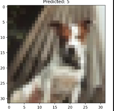
I randomly selected an image from the test set and had the model make a prediction. In this case, the model predicted class 5 (dog), and the actual class was also class 5, which was correct.

# Random image from the test set
random_idx = np.random.randint(0, len(X_val))
random_image = X_val[random_idx]

# Make prediction
prediction = model.predict(np.expand_dims(random_image, axis=0))
prediction_class = np.argmax(prediction, axis=1)

# Print the actual and predicted class
print(f"Actual Class: {np.argmax(y_val[random_idx])}")
print(f"Predicted Class: {prediction_class[0]}")

# Display the image with the predicted class
plt.imshow(random_image)
plt.title(f"Predicted: {prediction_class[0]}")
plt.show()

Outout:

Prediction array: [[6.4272822e-06 1.4340281e-07 5.5310270e-03 6.6405848e-02 4.2907866e-03
  8.9277107e-01 1.0174847e-03 2.9964956e-02 3.4941979e-07 1.2036602e-05]]
Actual Class of the random image: 5
Prediction class: 5

The model predicted correctly for this example, but there were cases where it made mistakes (e.g., predicting class 2 instead of 4).

Model Performance:

Validation Accuracy: ~71%
The model performed reasonably well, with training and validation accuracy steadily improving over the 10 epochs. The loss values for both the training and validation sets decreased, and there was no sign of overfitting.

Gratitude

This was the first problem on CNN and the second in deep learning. I’m finding it a bit complex to digest in a single day. As I mentioned yesterday, I plan to take on another challenge focused on deep learning after completing this one. And let’s be honest, I can’t wait to wrap up this challenge and reward myself with a delicious dinner—because coding deserves a tasty celebration!"

Stay Tuned!