Day 30 - Capstone Project: Predicting Loan Approvals Using Ensemble Learning (Random Forest, XGBoost)
On Day 30, the final day of the 30-day machine learning challenge, I tackled the Capstone Project: Predicting loan approvals using ensemble learning with two powerful models—Random Forest and XGBoost. Ensemble learning combines the predictive power of multiple models to improve performance and accuracy.
If you want to see the code, you can find it here: GIT REPO.
Dataset:
I used the Loan Approval Prediction Dataset from Kaggle, which contains various features such as Applicant Income, Loan Amount, Loan Term, Education, Self-Employment Status, and Loan Status (approved or rejected). The goal was to predict whether a loan will be approved or rejected.
Steps Taken:
Step 1: Load the Data
- I loaded the dataset and checked for any missing values and inconsistencies. The dataset didn’t have any missing values, but I noticed that some columns and values had extra spaces, which were removed for consistency.
Step 2: Preprocessing the Data
- I cleaned up the column names and values by stripping the leading and trailing spaces from the features.
- I used One-Hot Encoding to convert categorical features such as Education and Self-Employed into numerical values.
- The target column, Loan Status, was converted into 0 for “Rejected” and 1 for “Approved” for consistency.
Step 3: Splitting the Data
- I split the dataset into training and validation sets (80% training, 20% validation).
Step 4: Model Training
- Random Forest:
- I trained the Random Forest model using 100 decision trees. Each tree makes a prediction based on a random subset of data, and the final prediction is made based on the majority vote.
- XGBoost (Extreme Gradient Boosting):
- I trained the XGBoost model with a learning rate of 1.1 and 100 boosting iterations. XGBoost sequentially builds trees, each correcting the errors made by the previous ones.
- Random Forest:
Step 5: Model Evaluation
Both models performed exceptionally well, with 98% accuracy on the validation set. Here’s a breakdown of their performance:
Random Forest:
- Accuracy: 97.89%
- Confusion Matrix: [[309, 9], [9, 527]]
- Precision/Recall: Both models achieved nearly equal precision and recall, with a balanced performance across both approved and rejected loans.
XGBoost:
- Accuracy: 97.89%
- Confusion Matrix: [[310, 10], [8, 526]]
- Precision/Recall: XGBoost showed slightly better recall on rejected loans, making it just as effective as Random Forest.
Step 6: Visualization
- I plotted the confusion matrices for both models using heatmaps, which showed how well each model predicted approved and rejected loans.
Code Implementation:
import pandas as pd
from sklearn.model_selection import train_test_split
from sklearn.ensemble import RandomForestClassifier
from xgboost import XGBClassifier
from sklearn.metrics import accuracy_score, confusion_matrix, classification_report
import matplotlib.pyplot as plt
import seaborn as sns


# Step 1: Load the data.
data = pd.read_csv('dataset/loan_approval_dataset.csv')
# print(data.info())
# print(data.head())

# Step 2: Preprocess the data
# Check for missing values
#print(data.isnull().sum()) # We do not have any missing values.

# Find the categorical data.
# print(data[' education'].unique()) # [' Graduate' ' Not Graduate']
# print(data[' self_employed'].unique()) # [' No' ' Yes']
# print(data[' loan_status'].unique()) # [' Approved' ' Rejected']

# The dataset has an extra space before the actual value.
# Update the column name first.
data.columns = data.columns.str.strip()

# Now the values.
data['education'] = data['education'].str.strip()
data['self_employed'] = data['self_employed'].str.strip()
data['loan_status'] = data['loan_status'].str.strip()

# Convert the categorical data into numeric using One-Hot Encoding
data = pd.get_dummies(data, columns=['education', 'self_employed'], drop_first=False)

# For consistency, model expects in 0, 1. Change Rejected as 0 and Approved as 1
data['loan_status'] = data['loan_status'].replace({'Approved': 1, 'Rejected': 0}) # [1 0]

# Create features and Target Dataset
X = data.drop('loan_status', axis=1)  # Feature Dataset
y = data['loan_status']  # Target Dataset

# Step 3: Split the datasets into training and validation datasets.
X_train, X_val, y_train, y_val = train_test_split(X, y, test_size=0.2, random_state=42)

# Step 4: Build and Train the Models

# Random Forest Model
# How it works: It creates multiple decision trees on different subsets of the data, and each tree gives a prediction.
# The final prediction is based on the majority vote (classification) or the average (regression) of all the trees.
model_rf = RandomForestClassifier(n_estimators=100, random_state=42)
model_rf.fit(X_train, y_train)

# XGBoost (Extreme Gradient Boosting):
# How it works: XGBoost adds trees one by one, with each tree attempting to minimize the errors made by the previous
# trees using a gradient descent approach. It uses boosting techniques to improve performance.
model_xgb = XGBClassifier(n_estimators=100, learning_rate=1.1, random_state=42)
model_xgb.fit(X_train, y_train)

# Step 5: Make Predictions and Evaluate
# Random Forest
predictions_rf = model_rf.predict(X_val)

accuracy_score_rf = accuracy_score(predictions_rf, y_val)
confusion_matrix_rf = confusion_matrix(predictions_rf, y_val)
classification_report_rf = classification_report(predictions_rf, y_val)

print("Random Forest: ")
print(f"Accuracy Score: {accuracy_score_rf}")
print(f"Confusion Matrix: {confusion_matrix_rf}")
print(f"Classification Report: {classification_report_rf}")

# XGBoost
predictions_xgb = model_xgb.predict(X_val)

accuracy_score_xbg = accuracy_score(predictions_xgb, y_val)
confusion_matrix_xgb = confusion_matrix(predictions_xgb, y_val)
classification_report_xgb = classification_report(predictions_xgb, y_val)

print("XGBoost: ")
print(f"Accuracy Score: {accuracy_score_xbg}")
print(f"Confusion Matrix: {confusion_matrix_xgb}")
print(f"Classification Report: {classification_report_xgb}")

# Step 6: Visualization
plt.figure(figsize=(7, 5))
sns.heatmap(confusion_matrix_rf, annot=True, fmt='d', cmap='Blues', xticklabels=['Approved', 'Rejected'], yticklabels=['Approved', 'Rejected'])
plt.xlabel('Predicted Values')
plt.ylabel('Actual Values')
plt.title('Random Forest Confusion Matrix')


plt.figure(figsize=(7, 5))
sns.heatmap(confusion_matrix_xgb, annot=True, fmt='d', cmap='Blues', xticklabels=['Approved', 'Rejected'], yticklabels=['Approved', 'Rejected'])
plt.xlabel('Predicted Values')
plt.ylabel('Actual Values')
plt.title('XGBoost Confusion Matrix')

plt.show()
HeatMap
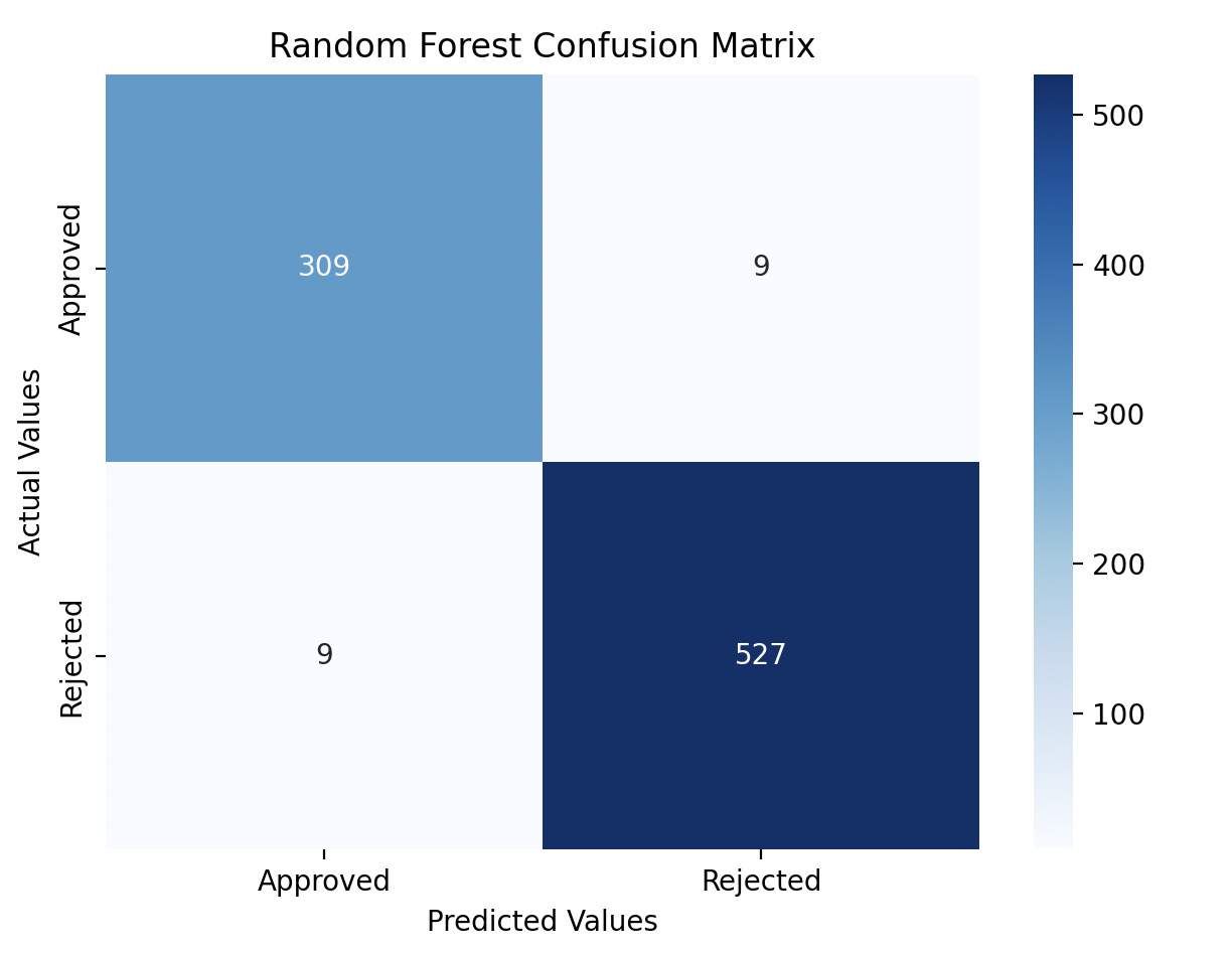
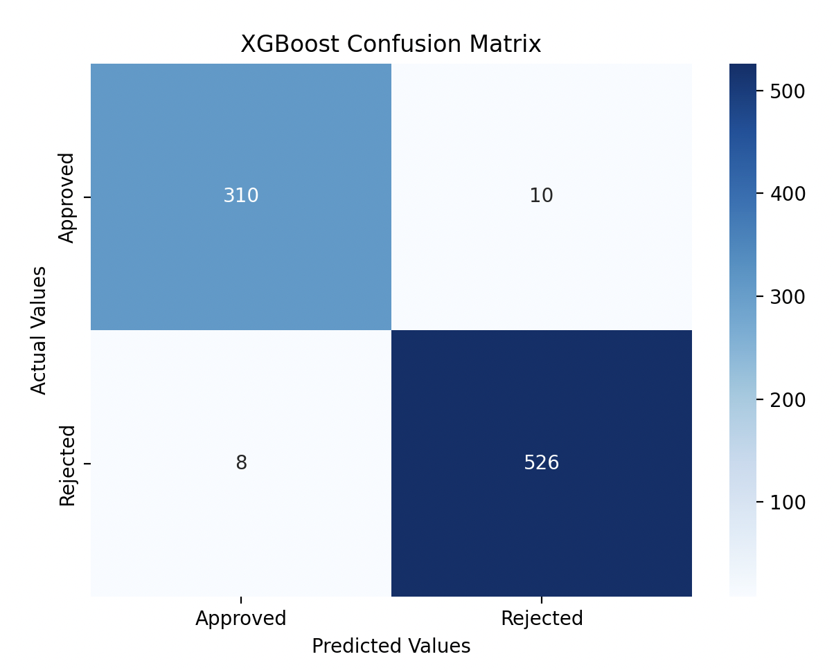
Both Random Forest and XGBoost delivered excellent results, each achieving 98% accuracy. The confusion matrix heatmaps made it easy to see how well each model predicted both approved and rejected loans, with only minor differences between the two models.
Gratitude:
This project wraps up the 30-day Machine Learning challenge! 🎉 It’s been such a great experience—it really helped me stay consistent, and seeing all the compiled code made me feel super productive. Setting a measurable goal like this was awesome, and I’m so pumped about the outcomes that I’m planning to take on even more!
While tackling the problems, I realized I had a tough time with the Deep Learning challenges. So, I’ve decided to dive into another adventure: the “30 Days, 30 Deep Learning Projects Challenge”!
I’m still working on the problem list and figuring out how it’ll all come together, but I’ll have all the details ready soon.
Stay tuned for the next chapter!