Day 7 - 30 Days 30 Machine Learning Projects
Hey, it’s Day 7 of the 30 Day 30 Machine Learning Projects Challenge. Today’s task was to build a model that predicts whether a customer will default on their credit card payment using a Random Forest Classifier. This is the first problem that uses Random Forest, so let’s explore how it works.
If you want to go straight to the code, I’ve uploaded it to this repository GIT REPO
The Problem
Determine Credit Card defaults using a Random Forest Classifier
We are trying to predict if a customer will default on their credit card payment based on several features, such as their payment history, bill amount, and limit balance. The dataset provides various customer attributes, and the target is whether they defaulted or not.
What is a Random Forest Classifier?
A Random Forest Classifier is a powerful ensemble learning method that builds multiple decision trees and combines their results. Each tree is trained on a random subset of data, and the final prediction is made by averaging the predictions of all trees (in classification tasks, it’s often the majority vote).
Imagine you’re asking several friends for their opinion about something. The more friends you ask, the more confident you’ll feel about the decision. That’s how Random Forest works—each “friend” (or tree) gives their opinion, and you trust the majority.
Understanding the Data
We used the Credit Card Default Dataset from Kaggle, which contains details about customers’ financial behavior. The target variable is whether or not they defaulted on their credit card payment. Unzip and put it in the dataset directory at the root level of your project.
Code Workflow
The process was divided into several steps:
- Load the data
- Preprocess the data
- Split the Data
- Create and train the Random Forest model
- Make predictions and evaluate
- Visualization
Step 1: Load the Data
I loaded the credit card dataset using pandas:
data_df = pd.read_csv('dataset/UCI_Credit_Card.csv')
Step 2: Preprocess the data
We separated the features (customer financial attributes) from the target (whether they defaulted or not):
X = data_df.drop('default.payment.next.month', axis=1) # Features
y = data_df['default.payment.next.month'] # target
Step 3: Split the Data
We divided the data into an 80-20 ratio: training (80%) and validation (20%) sets using:
X_train, X_val, y_train, y_val = train_test_split(X, y, test_size=0.2, random_state=42)
Here, random_state=42 sets the seed for randomness. This ensures the same split occurs on every run. The number 42 is commonly used but has no special meaning.
Step 4: Create and Train the model
I used a Random Forest Classifier with 100 trees (n_estimators=100) to train the model:
model = RandomForestClassifier(n_estimators=200, random_state=42)
model.fit(X_train, y_train)
The Random Forest learns patterns in the data by building multiple decision trees. Each tree learns from different parts of the data, and the final prediction is made by combining the results of all trees.
Step 5: Make Prediction and Evaluate
After training, I used the model to predict whether customers in the test set will default. I evaluated the model using the accuracy score, confusion matrix, and classification report.
predictions = model.predict(X_val)
accuracy_score = accuracy_score(y_val, predictions)
print("Accuracy score:\n", accuracy_score)
confusion_matrix = confusion_matrix(y_val, predictions)
print("Confusion Matrix:\n", confusion_matrix)
classification_report =  classification_report(y_val, predictions)
print("Classfication Report:\n", classification_report)
Step 6: Visualization
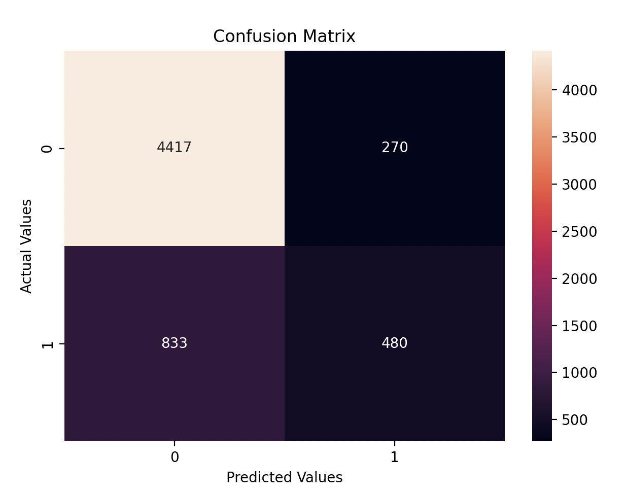
Finally, I visualized the confusion matrix to see how well the model performed on each class:
plt.figure(figsize=(10, 7))
sns.heatmap(confusion_matrix, annot=True, fmt='d')
plt.xlabel('Predicted Values')
plt.ylabel('Actual Values')
plt.title('Confusion Matrix')
plt.show()
Model Performance
The model achieved an accuracy of 81%, which is quite good for this dataset. However, let’s break it down further:
- True Positives (TP): Correctly predicted defaults are 480.
- True Negatives (TN): Correctly predicted non-defaults 4417.
- False Positives (FP): Customers predicted to default but didn’t are 270.
- False Negatives (FN): Customers predicted not to default but actually did 833.

Here’s the classification report that provides detailed precision, recall, and F1-scores:
               precision    recall  f1-score   support

           0       0.84      0.94      0.89      4687
           1       0.64      0.37      0.47      1313

    accuracy                           0.82      6000
   macro avg       0.74      0.65      0.68      6000
weighted avg       0.80      0.82      0.80      6000
Improvement
We can potentially improve the accuracy by tunning the model:
Hyperparameter Tuning: Random Forests have several parameters, like the number of trees (n_estimators), maximum depth (max_depth), minimum samples per leaf (min_samples_leaf), etc. Tuning these can improve performance.
model = RandomForestClassifier(n_estimators=400, max_depth=20, min_samples_leaf=8, random_state=42)Feature Importance: Check which features contribute the most using feature_importances_. You can try feature selection to remove irrelevant features and possibly improve the model.
Handling Class Imbalance: If your dataset is imbalanced (imbalance occurs when one class is significantly more frequent than the other, which can bias the model toward the majority class."), you can adjust class weights using class_weight=‘balanced’ in the RandomForestClassifier to give more weight to the minority class.
Key Takeaways
- Random Forest is a robust algorithm that performs well in classification tasks like predicting credit card defaults.
- Scaling isn’t required for Random Forest, but hyperparameter tuning and handling class imbalance can improve the results.
- The model shows good accuracy but struggles a bit with classifying the minority class (defaults). In future projects, I will experiment with class balancing techniques to improve this.
Gratitude
Today was a great learning experience with Random Forests. I can’t wait to finish this challenge and see everything I’ve learned.
Stay Tuned!