Day 2 - 30 Days 30 Machine Learning Projects

Thu, Sep 12, 2024
3-minute read

Hey, it is day 2 day of the 30 days 30 ML projects challenge. I got up at 5:30 am, which was again 30 minutes late than the target.

If you want to go straight to the code, I’ve uploaded it to this repository GIT REPO

Flow

The process for solving the problem is going to be the same. I ask ChatGPT for a solution and decode each line by asking follow-up questions. You can find the video of me coding it live at the bottom.

Straight to Problem, Please!

The challenge for day two was to “Classify Iris flowers into species using Logistic Regression”. It’s a classification problem.

Required Packages:

pip install pandas scikit-learn matplotlib numpy seaborn

Understand the Data

I am using the Iris dataset from the scikit-learn package. It consists of 50 samples from each of three species of Iris (Iris setosa, Iris virginica, and Iris versicolor), with four features describing the lengths and the widths of the sepals and petals.

   sepal length (cm)  sepal width (cm)  petal length (cm)  petal width (cm) species
0                5.1               3.5                1.4               0.2  setosa
1                4.9               3.0                1.4               0.2  setosa
2                4.7               3.2                1.3               0.2  setosa
3                4.6               3.1                1.5               0.2  setosa
4                5.0               3.6                1.4               0.2  setosa

Workflow of the Code

The workflow is divided into seven steps:

Loading the dataset
Preparing the data
Splitting the dataset
Training the model
Making predictions
Evaluating the model
Visualizing the evaluation results

Let’s dive into each step:

Step 1: Load the Dataset

Using the Iris dataset from the scikit-learn package, then converting it into a Pandas DataFrame for ease of manipulation.

iris = load_iris()
iris_df = pd.DataFrame(iris.data, columns=iris.feature_names)
iris_df['species'] = pd.Categorical.from_codes(iris.target, iris.target_names)

Step 2: Select Features and Target

The DataFrame consists of sepal and petal measurements. We’ll use these as features (X) to predict the species or the class (y).

Step 3: Split the Dataset

I split the data into a training set (80%) and a validation set (20%).

Step 4: Create and Train the Model

I initialized a LogisticRegression model and set max_iter to 200 so that the training process would converge properly. The higher the max_iter count, the better the chances of minimizing the loss function.

Step 5: Making Predicton

Now, make predictions on the validation data (X_val).

Step 6: Evaluating the model

For classification problems, relying solely on accuracy may not be sufficient. Therefore, we use a Confusion Matrix to better judge the performance. This will help us cover True Positive, False Positive, True Negative and False Negative of the prediction.

Here is the output:

Accuracy is:
 1.0

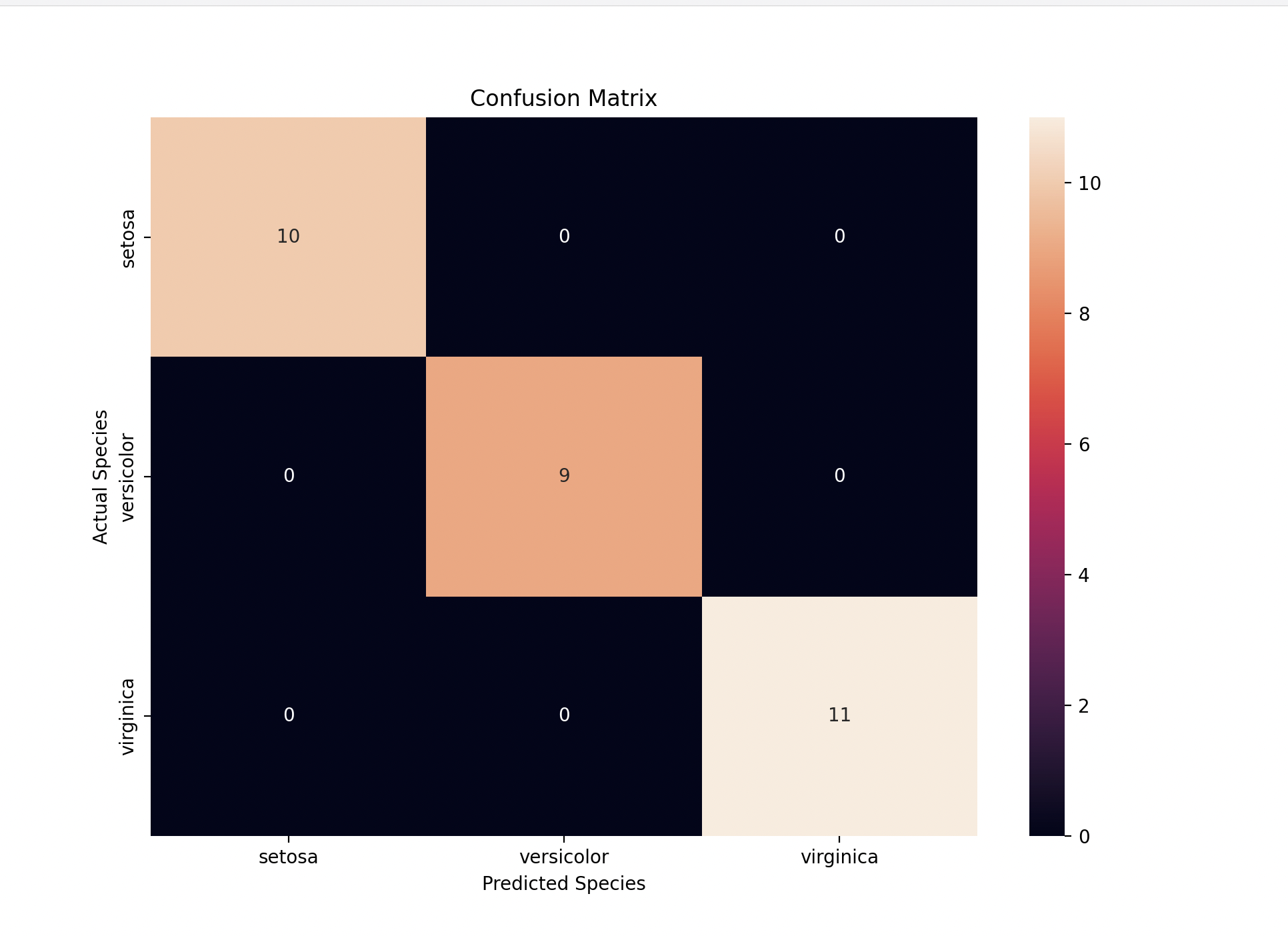
Confusion Matrix is:
 [[10  0  0]
 [ 0  9  0]
 [ 0  0 11]]

Classification report is:
               precision    recall  f1-score   support

      setosa       1.00      1.00      1.00        10
  versicolor       1.00      1.00      1.00         9
   virginica       1.00      1.00      1.00        11

    accuracy                           1.00        30
   macro avg       1.00      1.00      1.00        30
weighted avg       1.00      1.00      1.00        30

Step 6: Visualization

I used seaborn to create the heatmap of the Confusion Matrix, and this is how it looks:

Gratitude

I finished in 1 hour, which was faster than I planned. However, there were many new topics, like the Confusion Matrix, which I did not understand well. I read more about it in detail later in the day.

Below are the good source you can use:

Stay Tuned!!

Video

Posts in this series

30-days-ml-challenge