Day 3 - 30 Days 30 Machine Learning Projects

Fri, Sep 13, 2024
4-minute read

Good Morning! It is Day 3 of the 30 Day 30 Machine Learning Projects Challenge, and it is going great. I woke up at 5:17. All credit goes to my cat, Green, for scratching my head with his paws for his morning hunt. :)

If you want to go straight to the code, I’ve uploaded it to this repository GIT REPO

The flow is going to be the same as I had briefly explained in the Day 1 and Day 2 progress posts. I will be using ChatGPT and moving forward with follow-up questions.

Talk about the Problem Please!

The problem of the day was “Recognizing handwritten digits with k-Nearest Neighbors on MNIST”. It is another classic machine learning problem. Here, we have to predict handwritten digits using the K-Nearest Neighbors Algorithm. It also requires using MNIST data.

Wikipedia: The MNIST database (Modified National Institute of Standards and Technology database) is a large database of handwritten digits that is commonly used for training various image processing systems.

Undestanding the Data

I used the data from scikit-learn’s datasets fetch_openml with arguments:

mnist_784: This indicates that we want the MNIST data in which 28x28 size images are flattened into 784-feature vectors.
version=1: I specified that I wanted version 1 of the MNIST data.
as_frame=True: I specified that I wanted it in Panda DataFrame format, as it is easier to debug, visualize, and manipulate Panda DataFrames.
parser='auto': On my local machine, I was getting a warning about the parser version, so I set it to auto to pick the one that works best for the environment.

Code Workflow

The workflow is divided into seven steps:

Load the MNIST data
Preprocess the Data
Normalize the Data
Split data in training and validation sets
Create and Train Model
Make Predictions and Evaluate
Visualization

Let’s understand each step:

Step 1: Load the MNIST data

I have already mentioned in brief that I am using fetch_openml. See the Understand the Data section.

Step 2: Preprocess the Data

I had mentioned in Step 1 to load the data as Panda DataFrame, I use mnist_data.keys() to know about the list of keys the data contains. It has the following fields:

dict_keys(['data', 'target', 'frame', 'categories', 'feature_names', 'target_names', 'DESCR', 'details', 'url'])

I used the data and target to build my features (X) and target (y) sets.

Step 3: Normalize the Data

When dealing with image data, pixel values can range from 0 to 255 for 8-bit grayscale images. Normalizing these pixel values to the range between 0 and 1 is a common preprocessing step in machine learning tasks, particularly for algorithms that are sensitive to the scale of the input data, like k-Nearest Neighbors (k-NN).

I did X /= 255.0

Step 4: Split data.

I divided the data into an 80-20 ratio, that is, traning (80%) and validation (20%) sets using train_test_split(X, y, test_size=0.2, random_state=42)

Here random_state=42 is used to set the seed for randomness. It will ensure that the same split occurs on every run. The number 42 is a commonly used arbitrary number.

No logic behind it.

Step 5: Create and Train Model

I am using KNeighborsClassifier from scikit-learn neighbors package.

k-NN is a simple, instance-based learning algorithm that classifies new cases based on the majority votes of the k nearest neighbor samples from the training dataset. The ’nearest neighbors’ are determined by a distance metric, typically Euclidean distance. Here, K is user-defined.

Initially, I chose K=3.

Step 6: Make Predictions and Evaluate

I used a variable named predictions to store the predicted values against the 20% validation data X_val.

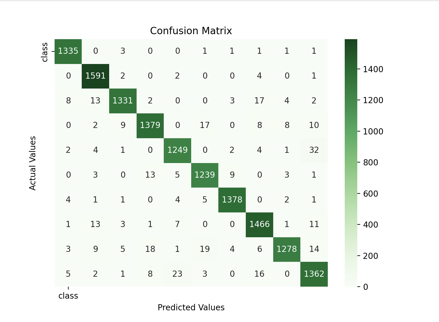
Since it is a classification type of model, relying on accuracy alone is not sufficient. I used a Confusion Matrix to learn more about the efficiency of the model.

A Confusion Matrix is helpful because it shows True Positives, False Positives, True Negatives, and False Negatives. I know it can be a little difficult to understand; please use the resources mentioned below to grasp it better.

Visualization

I used matplotlib.pyp and seaborn to create a heatmap of the confusion matrix. See how it looks.

Outcome of Experimenting with Different K.

At K=3, Accuracy: 0.9712857142857143
At K=2, Accuracy: 0.9642142857142857
At K=1, Accuracy: 0.972
At K=5, Accuracy: 0.9700714285714286
At K=10, Accuracy: 0.9657857142857142

I decided to stick with K=3.

Gratitude

Today, I was feeling confident writing the code and using libraries. It is the second problem on classification; maybe that has helped. I solved it in under 40 minutes, but then I started experimenting with different K values. It was fun. I am now enjoying the process and looking forward to solving more problems.

Stay Tuned!!

Posts in this series

30-days-ml-challenge