Day 4 - 30 Days 30 Machine Learning Projects

Sat, Sep 14, 2024
4-minute read

Good Evening! It’s Day 4 of the 30 Day 30 Machine Learning Projects Challenge. I went to the Ganesh Festival Heritage walk in the morning, so I only had time to solve the problem late in the evening.

If you want to go straight to the code, I’ve uploaded it to this repository GIT REPO

The process will be the same as I briefly explained in the Day 1-3 progress posts. I’ll use ChatGPT and ask follow-up questions.

Talk about the Problem Please!

Today’s problem was “Diagnose breast cancer as malignant or benign using a Decision Tree”. This is the third classification problem in a row. Today we’ll use a model called a “Decision Tree”.

ChatGPT Explains: A Decision Tree is like a flowchart that helps you make decisions step by step. It’s a tool used in machine learning to classify things or predict outcomes based on certain conditions.

Imagine This:

You want to decide whether a fruit is an apple or an orange.
You start asking simple yes or no questions. For example:
Is the fruit round?
If yes, ask: Is the fruit orange in color?
If yes → It's an orange.
If no → It's an apple.
If no → It’s something else, not an apple or orange.

Undestanding the Data

For this problem, you can use the Breast Cancer Wisconsin Dataset, which is often used for classification tasks. It’s available in Scikit-learn’s datasets module, so we don’t need to download it separately.

Code Workflow

The workflow is divided into six steps:

Load the dataset
Create feature and target set.
Split data in training and validation sets
Create and Train Model
Make Predictions and Evaluate
Visualization

Let’s understand each step:

Step 1: Load the dataset

Use load_breast_cancer() from sklearn.datasets

data = load_breast_cancer()

Step 2: Preprocess the Data

We can use the data as is. But I prefer to load it into a Pandas DataFrame. This helps manage datasets, especially for handling and visualizing data before training the model.

We can use data.keys() to see the list of keys the data contains. It has these fields:

dict_keys(['data', 'target', 'frame', 'target_names', 'DESCR', 'feature_names', 'filename', 'data_module'])

First, we create DataFrames using: X = pd.DataFrame(data.data, columns=data.feature_names) And store the target in: y = data.target

Step 3: Split data.

I divided the data into an 80-20 ratio: training (80%) and validation (20%) sets using: train_test_split(X, y, test_size=0.2, random_state=42)

Here, random_state=42 sets the seed for randomness. This ensures the same split occurs on every run. The number 42 is commonly used but has no special meaning.

Step 4: Create and Train Model

Use DecisionTreeClassifier from sklearn.tree. Then train it on X_train and y_train dataset.

Step 5: Make Predictions and Evaluate

I used a variable named predictions to store the predicted values for the 20% validation data X_val.

For diagnosing breast cancer, accuracy alone isn’t enough. We must use a Confusion Matrix for evaluation. It gives a more detailed view of the model’s performance, showing:

True Positives (TP): Correctly predicted malignant cases.
True Negatives (TN): Correctly predicted benign cases.
False Positives (FP): Benign cases incorrectly predicted as malignant (also known as Type I error).
False Negatives (FN): Malignant cases incorrectly predicted as benign (also known as Type II error).

Using a Confusion Matrix is important because:

Accuracy Alone is Not Enough: Accuracy tells you the percentage of correct predictions, but in cases where one class is more frequent (e.g., more benign tumors than malignant), accuracy might be misleading.
Class Imbalance: Breast cancer data may have more benign cases than malignant ones, so the model could predict benign for all cases and still get a high accuracy score, but this would be a bad model.
Performance Insights: It helps to identify:
- How well the model is detecting malignant tumors (minimizing false negatives is critical in medical diagnoses).
- Whether the model is flagging too many benign cases as malignant (false positives).

For more information, check out these resources:

Our model’s performance:

Accuracy is:
 0.9473684210526315

Confusion Matrix:
 [[40  3]
 [ 3 68]]

 Classfication Report:
               precision    recall  f1-score   support

           0       0.93      0.93      0.93        43
           1       0.96      0.96      0.96        71

    accuracy                           0.95       114
   macro avg       0.94      0.94      0.94       114
weighted avg       0.95      0.95      0.95       114

Step 6: Visualization

I used matplotlib.pyp and seaborn to create a heatmap of the confusion matrix.

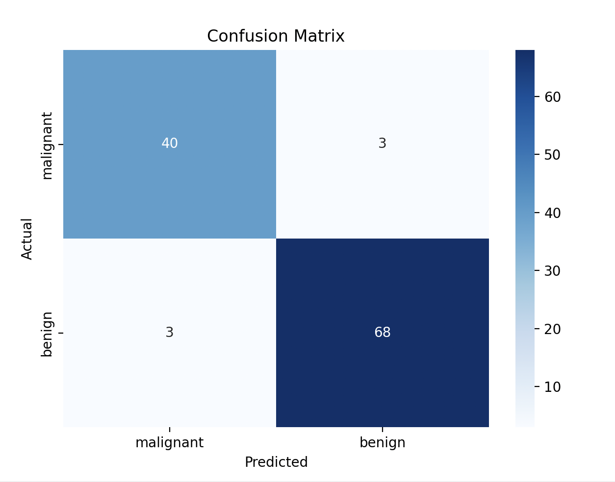
We can see the model predicts:

True Positives (TP): 40 correctly predicted malignant cases
True Negatives (TN): 68 correctly predicted benign cases

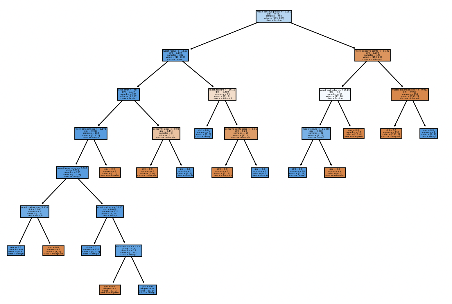
Let’s look at the descision tree:

Gratitude

It was a busy day, and I didn’t have time to solve the problem during the day. I finished all the work late at night. I’m extremely happy that the challenge streak is STILL ON. I’m looking forward to solving the next problem.

Stay Tuned!!

Posts in this series

30-days-ml-challenge