Day 5 - 30 Days 30 Machine Learning Projects

Sun, Sep 15, 2024
5-minute read

Good Morning, It’s Day 5 of the 30 Day 30 Machine Learning Projects Challenge.

If you want to go straight to the code, I’ve uploaded it to this repository GIT REPO

The process will be the same as I briefly explained in the previous progress posts. I’ll use ChatGPT and ask follow-up questions.

Talk about the Problem Please!

Today’s problem was “Filter spam from a collection of emails using Naive Bayes”. This is the fourth classification problem in a row. Today we will learn about Naive Bais Classifier.

Naive Bayes is a simple yet powerful algorithm often used for text classification. It uses probabilities to predict which class (spam or not spam) an email belongs to, based on the words in that email.

Here’s a simple analogy:

You have a box of fruits, and you know how often apples and oranges appear in that box. If someone hands you a fruit, you can guess whether it’s an apple or orange based on the features (like color or size). Similarly, Naive Bayes guesses whether an email is spam or not based on the frequency of certain words like “win,” “free,” or “meeting.”

Undestanding the Data

Since I didn’t have a large dataset initially, I created a small dataset of 20 emails (10 spam and 10 non-spam) to get started. Each email was labeled as either spam or ham (non-spam). Here’s a sample of that dataset:

Spam: “Win a $1000 Walmart gift card! Click here to claim now!”
Non-Spam: “Hey, are you coming to the meeting tomorrow?”

Code Workflow

The workflow is divided into six steps:

Create the Data
Preprocessing
Convert the text data into numerical features
Split data in training and validation sets
Create and Train Model
Make Predictions and Evaluate
Visualization

Let’s understand each step:

Step 1: Create the Data

I created a small dataset manually, using a dictionary to represent emails and their labels (spam or non-spam). For this small dataset, I used pandas to load the data into a DataFrame:

data = {
    'label': ['spam', 'ham', 'spam', 'ham', 'ham', 'spam', 'spam', 'ham', 'ham', 'spam',
              'ham', 'spam', 'ham', 'spam', 'ham', 'spam', 'spam', 'ham', 'spam', 'ham'],
    'email': [
        'Win a $1000 Walmart gift card! Click here to claim now!',
        'Hey, are you coming to the party tonight?',
        'Congratulations! You have won a free vacation to the Bahamas!',
        'Can we reschedule our meeting to 3 PM?',
        'Your Amazon order has been shipped.',
        'You have been selected for a cash prize! Call now to claim.',
        'Urgent! Your account has been compromised, please reset your password.',
        'Don’t forget about the doctor’s appointment tomorrow.',
        'Your package is out for delivery.',
        'Get rich quick by investing in this opportunity. Don’t miss out!',
        'Can you send me the latest project report?',
        'Exclusive offer! Buy one, get one free on all items.',
        'Are you free for lunch tomorrow?',
        'Claim your free iPhone now by clicking this link!',
        'I’ll call you back in 5 minutes.',
        'Get a $500 loan approved instantly. No credit check required!',
        'Hurry! Limited-time offer, act now to win a $1000 gift card.',
        'Let’s catch up over coffee this weekend.',
        'You’ve been pre-approved for a personal loan. Apply today!',
        'Meeting reminder for Monday at 10 AM.'
    ]
}

data_df = pd.DataFrame(data)

Step 2: Preprocess the Data

For binary classification, we mapped spam emails to 1 and non-spam (ham) emails to 0. This step allows the model to understand which class each email belongs to:

data_df['label'] = data_df['label'].map({'ham': 0, 'spam': 1})

Step 3: Convert the text data into numerical features.

Emails are in text form, so we need to convert them into numerical data. For this, I used the CountVectorizer from sklearn, which creates a matrix of word counts for each email (a “bag of words” model).

vectorizer = CountVectorizer(stop_words='english')
X = vectorizer.fit_transform(data_df['email']) # Convert the text into a bag of words matrix.

print("Vocabulary:\n", vectorizer.get_feature_names_out())
print("Count Matrix\n", X.toarray())

This transforms each email into a row of numbers, where each number represents how many times a word from the vocabulary appeared in that email.

Step 4: Split data

I divided the data into an 80-20 ratio: training (80%) and validation (20%) sets using:

X_train, X_val, y_train, y_val = train_test_split(X, data_df['label'], test_size=0.2, random_state=42)

Here, random_state=42 sets the seed for randomness. This ensures the same split occurs on every run. The number 42 is commonly used but has no special meaning.

Step 5: Create and Train Model

For this task, I used the Multinomial Naive Bayes model from sklearn. It’s particularly well-suited for text data:

model = MultinomialNB()
model.fit(X_train, y_train)

The model learned from the training data, looking at how often certain words (like “win,” “free,” or “meeting”) appeared in spam and non-spam emails.

Step 6: Make Predictions and Evaluate

After training, I used the model to predict whether the emails in the test set were spam or not. To evaluate the model’s performance, I calculated its accuracy and created a confusion matrix:

predictions = model.predict(X_val)
accuracy_score = accuracy_score(y_val, predictions)
print("Accuracy Score:\n", accuracy_score)
confusion_matrix = confusion_matrix(y_val, predictions)
print("\nConfusion Matrix:\n", confusion_matrix)

Accuracy alone doesn’t tell the full story. That’s why I also used a confusion matrix to get a better picture of how the model handled spam and non-spam emails.

Here’s a breakdown of the confusion matrix:

True Positives (TP): Correctly predicted spam emails.
True Negatives (TN): Correctly predicted non-spam emails.
False Positives (FP): Non-spam emails incorrectly predicted as spam.
False Negatives (FN): Spam emails incorrectly predicted as non-spam.

Our model’s performance:

Accuracy Score:
 1.0

Confusion Matrix:
 [[2 0]
 [0 2]]

Step 7: Visualization

I used matplotlib.pyp and seaborn to create a heatmap of the confusion matrix.

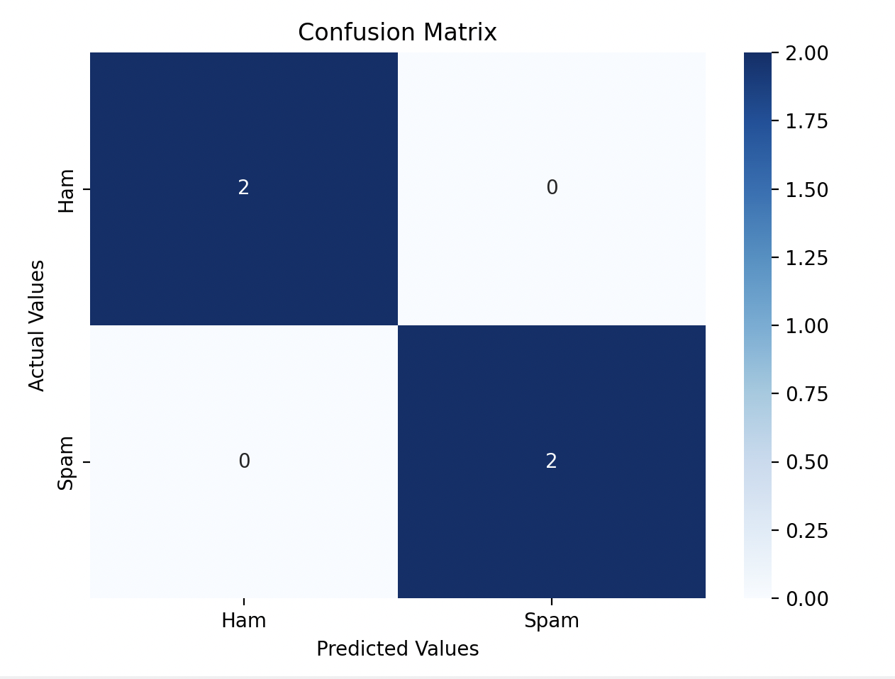
We can see the model predicts:

True Positives (TP): 2 correctly predicted spam emails
True Negatives (TN): 2 correctly predicted non-spam emails

Gratitude

The Naive Bayes algorithm is simple yet effective for text classification problems like spam filtering. While the model worked well on this small dataset. I will try it on larger dataset in future posts.

Stay Tuned!!

Posts in this series

30-days-ml-challenge