Day 9 - 30 Days 30 Machine Learning Projects

Thu, Sep 19, 2024
4-minute read

Problem: Forecasting weather with Simple Linear Regression on time series data

Hey, it’s Day 9 of the 330 Day 30 Machine Learning Projects Challenge. Today’s challenge was about forecasting weather using a Simple Linear Regression model. The goal was to predict future temperatures based on historical temperature data. Let’s break it down step-by-step and see how the model performed.

If you want to see the code, you can find it here: GIT REPO.

Understanding the Data

We used the Daily Temperature of Major Cities dataset from Kaggle. It contains temperature data from cities around the world, recorded daily. For this project, we filtered the data to focus on India and used Date and AvgTemperature (average temperature) as the primary columns for forecasting. Download, unzip and put it in the dataset directory at the root level of your project.

The data spans multiple years, and the challenge was to predict the temperature for future dates based on past data using a time series approach.

Step-by-Step Code Workflow

The code was broken down into the following steps:

Step 1: Load the Data

We started by loading the dataset using pandas. Since the data is large, we set low_memory=False to avoid mixed-type warnings during loading.

data = pd.read_csv('dataset/city_temperature.csv', low_memory=False)

Step 2: Filter Data for India

We filtered the dataset for India and removed any invalid temperature values (AvgTemperature > -99).

india_data = data[(data['Country'] == 'India') & (data['AvgTemperature'] > -99)].copy()

Step 3: Combine Date Columns

Next, we combined the Year, Month, and Day columns into a single Date column to create a proper time series.

india_data.loc[:, 'Date'] = pd.to_datetime(india_data[['Year', 'Month', 'Day']])

Step 4: Select Relevant Columns

We only kept the relevant columns — Date and AvgTemperature — for our analysis.

rel_india_data = india_data[['Date', 'AvgTemperature']]

Step 5: Preprocess the Data

We removed any missing values to ensure clean data, then converted the Date into a numeric format using ordinal numbers. This allowed our Linear Regression model to work with time as a feature.

rel_india_data = rel_india_data.dropna()
rel_india_data['Date_ordinal'] = rel_india_data['Date'].map(pd.Timestamp.toordinal)

Step 6: Train-Test Split

We split the data into training (80%) and validation (20%) datasets using train_test_split.

X_train, X_val, y_train, y_val = train_test_split(X, y, test_size=0.2, random_state=42)

Step 7: Build and Train the Model

We trained a Simple Linear Regression model using the training data. The model tries to fit a straight line to the relationship between time and temperature.

model = LinearRegression()
model.fit(X_train, y_train)

Step 8: Make Predictions and Evaluate

The model made predictions on the validation data. We evaluated its performance using Mean Squared Error (MSE), which measures how far the predicted values are from the actual values.

predictions = model.predict(X_val)
mean_squared_error = mean_squared_error(y_val, predictions)
print(mean_squared_error)

Step 9: Visualization

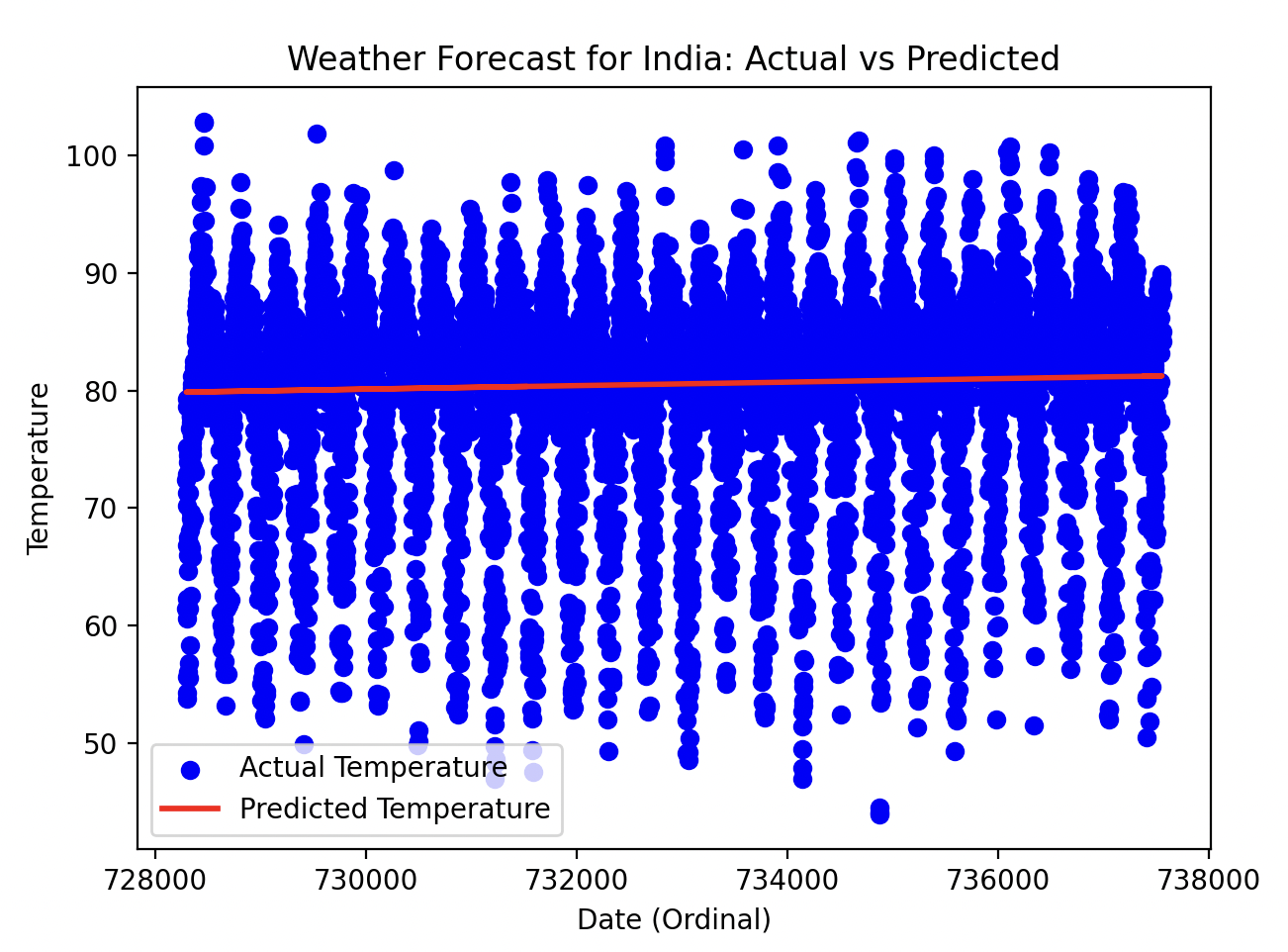
We visualized the model’s predictions against the actual temperatures. The blue dots represent actual temperatures, while the red line represents the predicted temperatures.

plt.figure(figsize=(7, 5))
plt.scatter(X_val, y_val, color='blue', label='Actual Temperature')
plt.plot(X_val, predictions, color='red', linewidth=2, label='Predicted Temperature')
plt.xlabel('Date (Ordinal)')
plt.ylabel('Temperature')
plt.title('Weather Forecast for India: Actual vs Predicted')
plt.legend()
plt.show()

Model Performance

The model achieved an accuracy of 74%, which is moderate. However, the performance is not ideal, as weather patterns can be very complex and linear models often fail to capture these trends accurately.

Prediction Line: The predicted temperatures were nearly constant, as seen in the plot. This is a limitation of the linear model, as it struggles to capture non-linear, seasonal trends in weather data.

What Can We Do?

To improve the forecast, here are a few options to explore:

Introduce Complexity: We might need more sophisticated models like Polynomial Regression (to capture nonlinear trends) or Time Series Models like ARIMA or Prophet, which can account for seasonal patterns.
Add More Features: Simple Linear Regression is based only on the date. Adding additional features, such as previous day’s temperature, humidity, or atmospheric pressure, might help the model capture more intricate weather patterns.

Key Takeaways

Simple Linear Regression can capture basic trends, but it struggles with complex data like weather forecasting.

Gratitude

Working on weather forecasting with time series data was a great experience. It highlighted the limitations of linear models for complex patterns like weather and gave me insight into how we can tackle such problems using more advanced techniques.

Stay tuned!

Posts in this series

30-days-ml-challenge